中文 EN

5.17.8.1. Revision History

The revision history lists the major changes between document versions. The table below outlines the technical content of each document update.

Version	Revision Date	Revision Notes
V0.1	2023-03-25	First compilation completed (Cmodel phase)
V0.2	2024-01-12	Overall structure compilation completed
V0.3	2024-03-09	Updated parameter list and descriptions
V0.4	2024-04-09	Adjusted document formatting
V0.5	2024-05-09	Updated parameter descriptions and debugging flowchart
V1.0	2024-06-17	Added 3A debugging instructions, revised some textual descriptions
V1.1	2024-09-04	Corrected formatting errors, improved AE/AWB/WDR ISP module function descriptions

5.17.8.2. X5 ISP Introduction

Overview

This document introduces the test and debugging methodology for the Horizon Sunrise X5 image processor, providing detailed explanations of systematic debugging methods for static images and dynamic video image quality. The debugging results are influenced by factors such as the CMOS sensor, lens optical performance, module structure, and image processor; therefore, in practical debugging, appropriate debugging strategies should be adopted based on hardware and specific project requirements.

Image quality testing should span the entire project development cycle, with targeted image quality optimization conducted at different stages. At least two comprehensive rounds of image quality evaluation and debugging should be performed during project development. Image evaluation testing requires a standardized laboratory environment to conduct precise objective assessments of image quality. The lab environment must include equipment capable of adjustable illuminance and color temperature to meet testing requirements under various lighting conditions.

This document includes descriptions related to objective image quality testing, which enables relatively accurate quantitative analysis of images. Some debugging procedures require specific lighting conditions and can be optimized through targeted comparisons with competitor camera objective data.

Subjective debugging requires testing under real-world scenarios. During testing, already-tuned effect parameters should be used across multiple scenarios, with fine-tuning based on test results. For camera products with special applications, targeted optimization and debugging are required according to their specific usage environments due to their unique application characteristics.

Subsequent sections of this document detail debugging and testing methods, debugging procedures, data analysis, and how to optimize ISP parameters based on data testing and analysis.

Horizon Sunrise X5 supports three modes: Linear, HDR, and Native-WDR-lin. This document primarily introduces image debugging for Linear mode. Debugging methods for non-Linear modes will be specially noted if applicable.

ISP Pipeline

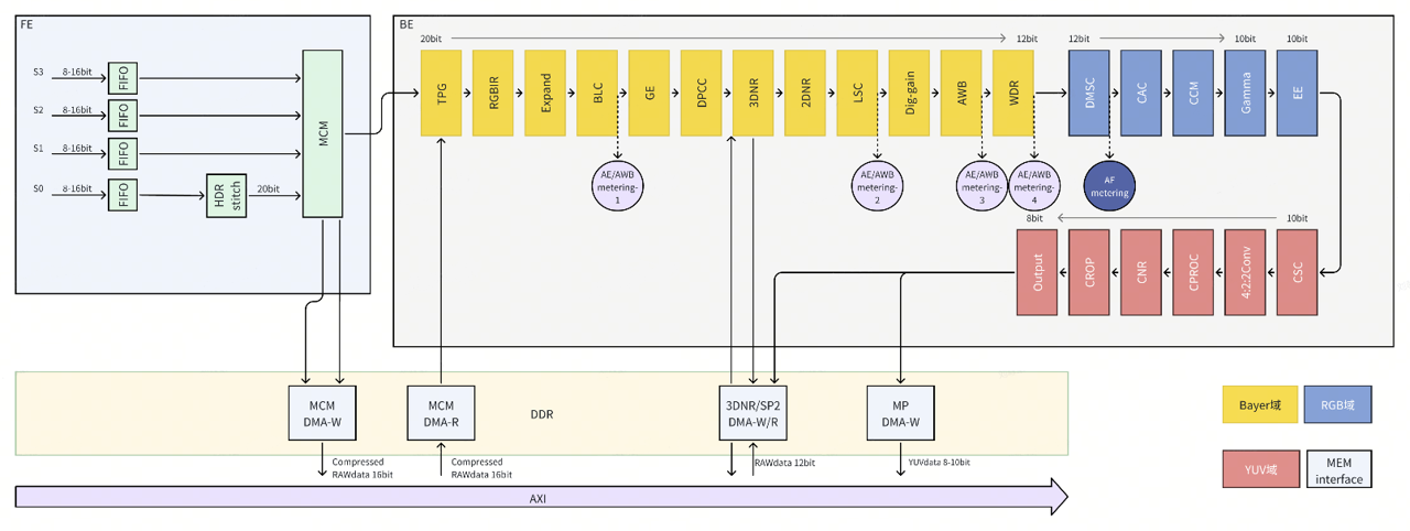
Figure 1.2‑1 Algorithm Module Flowchart

In the diagram, modules with yellow backgrounds represent processing in the RAW domain, those with red backgrounds represent processing in the RGB domain, those with blue backgrounds represent processing in the YUV domain, and light purple sections represent AE/AWB statistical calculations. The four positions indicated by dashed lines are optional statistical locations for AE/AWB, which can be switched according to actual needs.

5.17.8.3. ISP Tuning Overview

Tuning Procedure

Tuning Equipment

Debugging the image quality of Horizon X5 ISP requires preparing corresponding instruments based on actual application scenarios to ensure smooth debugging. The following are laboratory instruments and equipment required for typical scenario debugging of Horizon Sunrise X5 ISP:

• 24 X-Rite Color chart

• Edmund optics Opal diffusing glass

• ISO12233 chart

• ISO15739 chart

• 2 adjustable illuminance vertical light boxes

• Tripod and camera module mounting fixture

• Standard adjustable color temperature light box

• Studio scene

• Illuminance meter

• Exposure testing instrument

• DNP light box

• 36-step transmissive HDR testing instrument

Tuning in Phases

The ISP parameter calibration process mainly consists of three phases:

• Phase 1: Confirm that the CMOS sensor can be correctly initialized to obtain accurate RAW information and perform characteristic parameter configuration;

• Phase 2: Optimize and debug ISP-related algorithm modules based on sensor characteristics;

• Phase 3: Systematic testing and evaluation, comprehensive system-level debugging to meet image quality requirements across various scenarios.

Figure 2.1-1 shows the flowchart of the three debugging phases.

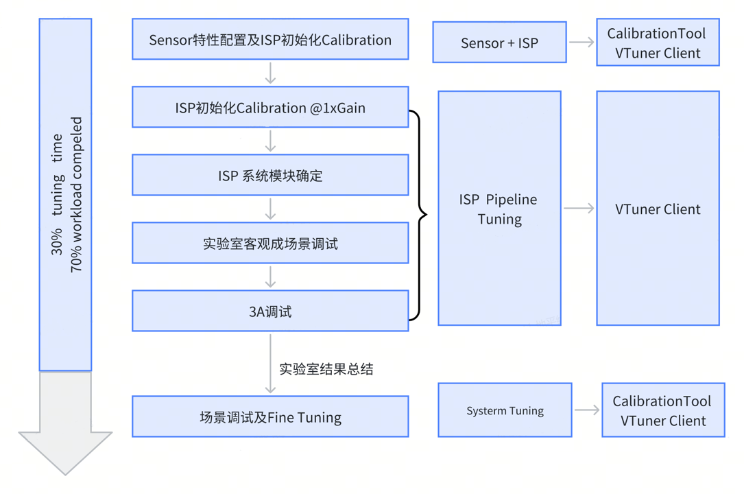
Figure 2.1‑1 ISP Tuning Process

Phase 1 - Sensor Dependent Calibration

Hobotplayer is a visualization tool integrating display and data capture functions, used during debugging to capture Raw and YUV data. In the early debugging phase, the Calibration Tool is used to configure sensor characteristics. Raw images are captured according to the debugging needs of each module, and static debugging parameters of the sensor are calibrated using the Calibration Tool. For usage instructions of the static Raw image capture tool Hobotplayer and the objective parameter calibration tool Calibration Tool, refer to “X5-Calibration Tool User Guide”.

Sensor characteristic configuration and optical characteristic correction require the following modules:

• Black Level Subtraction

• De-Companding (frontend/FE) LUTs. For WDR PWL mode

• Noise profile (NP)

• Green Equalization (GE)

• Dynamic dead pixel correction (Dynamic DPC)

• Auto-exposure (AE)

• Lens shading correction (LSC)

• Auto-white balance (AWB)

• Gamma

• Color correction matrix (CCM)

• Chromatic aberration correction (CAC)

• Purple fringe correction (PF)

Phase 2 - Algorithm

Debugging in the second phase depends on the characteristics of the CMOS sensor being debugged and the selected ISP algorithm mode, with corresponding parameters optimized according to lighting conditions. This phase is mainly implemented using the dynamic debugging tool VTunerClient. For usage instructions of VTunerClient, refer to “X5-VtunerClient Tool Guide”. Image quality is optimized according to scene requirements through systematic debugging of the following modules:

• Stitching

• 2DNR

• 3DNR

• Demosaic

• WDR (LTM)

• Color noise reduction (CNR)

• Edge Enhancement

• ISP modules

Phase 3 - Fine Tuning

Since parameters debugged in the first two phases may not cover all scenarios, some scenes might exhibit unsuitable or unacceptable image effects, requiring detailed optimization for specific scenes in the third phase. Generally, this phase requires different brightness and color temperature lighting conditions. Corresponding tests must be conducted under different lighting environments to evaluate whether the debugged parameters can cover a sufficient number of real-world scenarios. Image quality analysis requires comprehensive evaluation combining both subjective and objective aspects. For scenes requiring debugging, current image quality and parameters should be analyzed before re-debugging. Through repeated testing and debugging to determine the direction, key parameters improving issues are identified and appropriately optimized.

ISP modules typically requiring debugging in Phase 3 include:

• 2DNR strength

• 3DNR strength

• CNR strength

• WDR strength

• CCM module color saturation strength

• Demosaic

• EE strength

Note: During debugging across all three phases, any modifications after initialization may affect subsequent module performance, such as color reproduction, noise reduction, and image details, as shown in Figure 2.1-2. The corresponding solution is iterative debugging as illustrated. For example, if debugging the Black Level Subtraction module is required, since BLS is the first module in the ISP pipeline, it affects color, noise/detail, so all other modules need to be re-debugged.

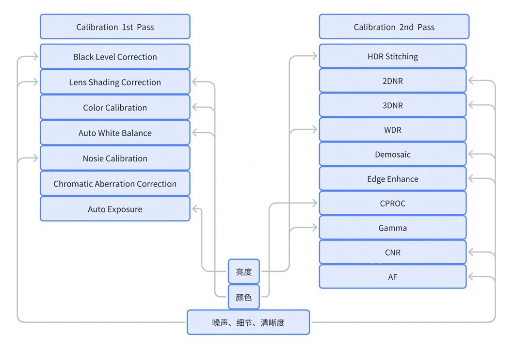
Figure 2.1‑2 Tuning Cycles

System Requirement for ISP Tuning

Before debugging, relevant equipment and environmental information must be verified:

ISP Information

• Product application scenarios and image quality requirements

• ISP debugging result delivery method

• ISP image processing block diagram

• Image processing application modes: Linear, HDR, Native-WDR-lin, etc.

• Input data format and bit depth

• Resolution and frame rate of images to be tuned

• Color pattern mode of the sensor being tuned

• Whether OTP parameters are needed

• Whether built-in ISP is available

Sensor Configuration Information

• High dynamic mode (HDR), sensor exposure ratio and exposure time constraints

• Wide dynamic mode (WDR), sensor datasheet and decompression node information

• Sensor configurable exposure and gain range

• Frame rates and resolutions supported by the sensor

• Data format output by the sensor

• Sensor raw data structure

Sensor Optical Information

• Evaluation of hardware performance consistency among module units

• Characteristics of infrared cut-off filter

• Black level temperature drift and whether it changes with analog gain

ISP Modes

The debugging process aims to determine the optimal values for parameters in each module of ISP image processing. These parameters are saved in corresponding files, which can be obtained from debugging tools Calibration Tool and VTunerClient. Main debugging parameter file descriptions are as follows:

Filename	Description
Sensor_Calibration.XML	Module calibration file containing data related to module characteristics such as BLC, LSC, CCM, WB, NoiseProfile, calibrated based on module RAW data
Sensor_Tuning.json	Debugging parameter configuration for each module in the ISP Pipeline, including parameter configurations in Manual and Auto modes and module calibration parameters

Table 2.2‑1 ISP Initial Debugging Configuration File Descriptions

Tuning Tools (Calibration Tool/VTunerClient)

Horizon X5 ISP uses two tools to assist in effect debugging: static calibration tool Calibration Tool and dynamic debugging tool VTunerClient.

Calibration Tool

The Calibration Tool is used to generate a static calibration file, which is needed during parameter integration and is generally named sensorName.json or sensorName.xml. This file contains tuning parameters related to the lens and sensor, such as black level, shading lookup tables, and parameters open for tuning in the AWB algorithm.

The primary goal of Phase 1 tuning is to calibrate and obtain the static calibration file using the Calibration Tool. This tool may also be used in later phases to correct previous calibration errors or issues.

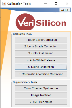
Figure 2.2‑1 Calibration Tool Main Interface

When using the Calibration Tool, modules can be calibrated sequentially according to the numbers on the interface, or individual modules can be run separately for parameter calibration. After calibration, the corresponding static calibration file is generated via XML Generator.

VTunerClient

VTunerClient can be used to modify effect parameters of each module, with the effect changes displayed in real-time on the frame shown by the Hobotplayer tool. On the VTunerClient debugging interface, effect parameters are categorized by functional modules, allowing parameter modifications within the corresponding module. After importing the effect file calibrated by the Calibration Tool, VTunerClient adjusts the parameters of the corresponding modules. After debugging, the current debugging parameters can be saved as a .json file. The VTunerClient interface is shown in Figure 2.2‑2.

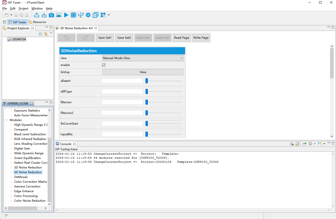
Figure 2.2‑2 VTunerClient Debugging Interface

Hobotplayer

Hobotplayer is a tool for real-time display of device frame, also used to save image data in different formats such as RAW, YUV, BMP, JPG. The Hobotplayer interface is shown in Figure 2.2‑3, with page parameter descriptions in Table 2.2-2. After setting the correct device IP and port in Init_config, click the connect button in the left function panel to view the data stream. To dump raw data, check raw_en, enter a natural number greater than 0 in the raw_num field, then check the save_raw box.

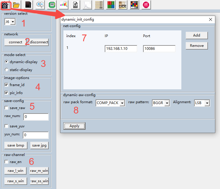
Figure 2.2‑3 Hobotplayer Interface

Module	Function	Description
version select (part 1 in Figure 2.2 3)	Select platform	Select corresponding platform
network (part 2 in Figure 2.2 3)	Network connect/disconnect	-
mode-select (part 3 in Figure 2.2 3)	Switch between network transmission/static display	Select dynamic-display for real-time data stream, select static-display to open static data
image-options (part 4 in Figure 2.2 3)	Display image information and frame number	-
save-config (part 5 in Figure 2.2 3)	Save raw or yuv	Enter a number in the raw_num/yuv_num field first, then check save_raw/save_yuv to save
raw-channel (part 6 in Figure 2.2 3)	Display raw image by channel	Raw image can be seen after checking raw_en, usually using raw_l_win
init_config (part 7 in Figure 2.2 3)	Configure network and port number	Development board network IP
Apply (part 8 in Figure 2.2 3)	Confirm configuration	-

Table 2.2‑2 Hobotplayer Initial Configuration Interface Description

5.17.8.4. ISP Tuning Modules

Auto-Exposure (AE)

Overview

Auto-Exposure (AE) accurately restores the current scene’s brightness by adjusting image brightness. Although AE plays a secondary role in characterizing sensor characteristics, it is one of the most fundamental critical modules throughout the ISP debugging process. AE adjustments can be made in three steps using VTunerClient.

• Phase 1: AE can be manually set when debugging other modules. This depends on each module’s exposure requirements, detailed in each module’s debugging documentation.

• Phase 2: Calibrate AE parameters for most scenes in the lab according to objective index requirements.

• Phase 3: Fine-tune AE parameters to suit all scenes. Main adjustments are based on parameters dynamically changing with gain.

Tuning Theory

The following figure shows the AE processing flowchart:

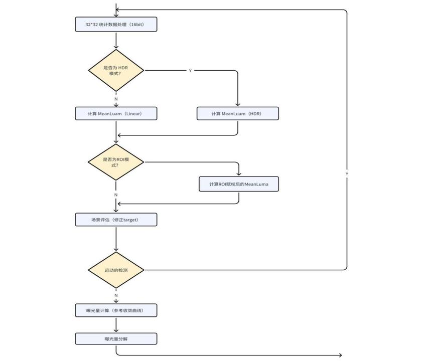
Figure 3.1‑1 AE Processing Flowchart

Statistical Positions

There are four statistical positions for AE in the pipeline, as shown in Figure 3.1-2.

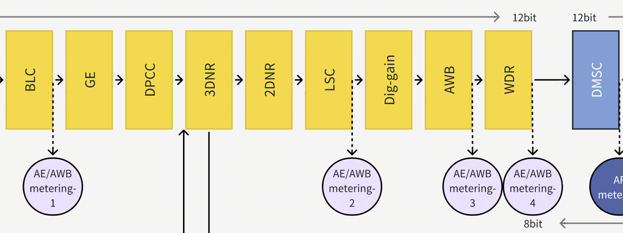
Figure 3.1‑2 AE Statistical Data Nodes

Data Storage and Processing

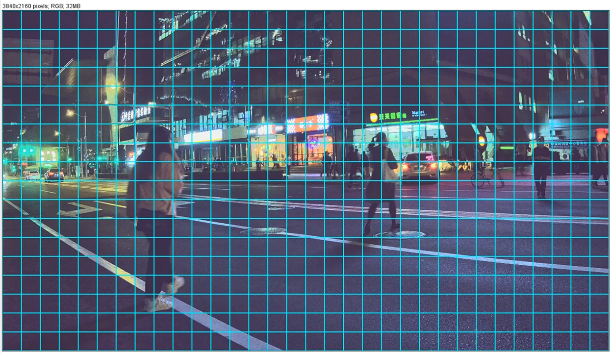
The general statistical module for ISP auto-exposure control divides the entire image into 32×32 blocks and calculates the average value for each channel (R, GR, GB, B). These averages are output as statistical data used to implement auto-exposure.

For each sub-block within the 32×32 statistical array, one 32-bit statistical data is output, containing average values for R, GR, GB, and B channels. The data structure of the statistical data is shown below. For HDR mode sensors, during statistical data processing, each block’s luminance value is multiplied by the HDR ratio.

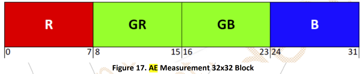
Figure 3.1‑3 AE/AWB Statistical Data Storage Format

Taking a 3840x2160 resolution image in linear mode as an example, the distribution of 32×32 windows in the image is shown below:

Metering Mode

Auto-exposure (AE) metering function divides the image into multiple blocks and calculates the image’s actual brightness by averaging the brightness of each block. The statistical grid covers the entire image to collect exposure-related statistical data. By configuring different numbers of Regions of Interest (ROI) and assigning weights to each ROI, AE metering modes can be adjusted to suit different application scenarios.

The following are different AE metering modes:

• (Default) Average metering. In this mode, the image is divided into 32 x 32 blocks, and image brightness is the average brightness of all blocks.

• ROI metering. In this mode, the image is divided into multiple blocks. The number of blocks is specified by roiNumber. Image brightness is determined by the image’s average brightness measured in average metering mode and the average brightness of all ROIs weighted by roiWeight. A higher roiWeight value places greater emphasis on ROI average brightness.

ROI metering includes the following operations:

• ROI configuration. By default, up to 25 ROI regions can be configured during initialization. These regions can be selected according to scene requirements. For example, if the subject to be photographed is at the center of theframe, the center area can be set as the ROI to ensure accurate subject exposure;

• Weight assignment. Weights for each ROI region and non-ROI regions can be configured separately. Weights determine the influence of that region in overall exposure calculation. For important areas, higher weights can be set to ensure they have a greater proportion in exposure calculation.

• Overlapping region handling: When ROI regions overlap with 32x32 blocks, the system overlays weights based on the proportion of the block covered by the ROI region. This means if a block only partially covers the ROI region, its weight in exposure calculation is adjusted according to the coverage ratio.

Debugging related parameters are shown in the table below:

Parameter	Type	Range	Description	Default Value
roiNumber	uint8_t	[0, 25]	The number of ROI regions.	0
roiWeight	float	(0, 1)	The weight of the average brightness of the ROI area, which is weighted against the overall average brightness of the entire image during metering.	0.5
roiWindow	Type: Vsi3ARoiWindow_t[25*5] where Vsi3ARoiWindow_t{float32_t fx; float32_t fy; float32_t fw; float32_t fh; float32_t weight}	Weight:[0, 255]; Others: changes with the image size	The ROI window position and size. l fx: the starting position of each ROI in the horizontal direction. l fy: the starting position of each ROI in the vertical direction. l fw: the width of each ROI. l fh: the height of each ROI. l weight: the weight of each ROI.	[0, 0, 100, 100, 1]
expV2WindowWeight	float[32*32]	[0, 255]	The weight of every block in the image.	1

Table 3.1‑1 Statistical Window ROI Configuration

Through this flexible configuration and weight assignment, AE metering can adapt to various complex application conditions, achieving more accurate auto-exposure. This is very important for improving image quality, especially in dynamically changing environments.

Scene Adaptation

Adaptive AE is an intelligent exposure technology used to adjust the target average brightness based on scene evaluation in backlit or low-light scenarios.

To use adaptive AE, scene evaluation must first be enabled. The setpoint value after adaptive AE processing is jointly determined by the setpoint value before adaptive AE processing and the compressed setpoint value, weighted by targetFilter. Basic adaptive AE parameters are listed in Table 3.1-2:

Parameter	Type	Range	Description	Default Value
semMode	enum	{CAMDEV_AE_SCENE_EVALUATION_FIX, CAMDEV_AE_SCENE_EVALUATION_ADAPTIVE}	Whether to enable the scene evaluation function. Value range: l CAMDEV_AE_SCENE_EVALUATION_FIX: disable scene evaluation. l CAMDEV_AE_SCENE_EVALUATION_ADAPTIVE: enable scene evaluation.	CAMDEV_AE_SCENE_EVALUATION_FIX
targetFilter	float	(0,1)	The weight to get the setPoint value after adaptive AE. The greater the parameter value, the more contribution the setPoint value before the processing of adaptive AE makes to the setPoint value after the processing of adaptive AE.	0.5

Table 3.1‑2 Basic Adaptive AE Parameters

Backlight Scene Compensation

Key parameters are listed in Table 3.1-3.

Parameter	Type	Range	Description	Default Value
wdrContrastMin	float	(0, 255)	The threshold c1 for determining normal exposure. If the brightness of the current frame is less than c1, the exposure is normal.	10
wdrContrastMax	float	(0, 255)	The threshold c2 for determining strong backlight. If the brightness of the current frame is greater than c2, the backlight is strong. If the brightness is less than c2 but greater than c1, the backlight is mild.	110

Table 3.1‑3 Backlight Compensation Parameters

If wdrContrastMin and wdrContrastMax are decreased (reducing the minimum and maximum values of backlight limitation), low-brightness areas in the image will significantly brighten, approaching the setpoint, but high-brightness areas may become overexposed.

If wdrContrastMin and wdrContrastMax are increased (increasing the minimum and maximum values of backlight limitation), the overall image brightness will approach the setpoint, with low-brightness areas slightly brightening while remaining relatively dim.

Low-Light Scene Compensation

The current frame’s low-light level depends on the frame’s exposure. The greater the exposure, the darker the illumination conditions, and the more the setpoint needs to be compressed.

Photos taken under low-light conditions often have more noise. If the setpoint is too large, the AE-adjusted image will be brighter, and noise will be amplified. Therefore, for lower ambient brightness, the setpoint should be appropriately compressed. AE supports dynamically adjusting the convergence target value in HDR/Linear modes under dark conditions to optimize image performance. The debugging methods for both modes are similar. The form of AE convergence target value changes under dark conditions after dynamic adjustment is shown in the figure below (using Linear mode as an example).

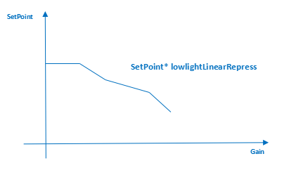
Figure 3.1‑4 AE Low-Light Compensation Logic Diagram

Table 3.1-4 lists parameters for adjusting target brightness under dark conditions in linear and HDR modes.

Parameter	Type	Range	Description	Default Value
lowlightLinearLevel	uint32_t	[0,16]	The number of nodes in the Gain / Repress array in linear mode.	4
lowlightLinearRepress	float[5]	[0,1]	The array of compression ratios for the target brightness that varies with the gain in linear mode.	[1.0, 0.8, 0.6, 0.4, 0.4]
lowlightLinearGain	float[5]	[0,255]	The array of key node values of the total gain of the sensor in linear mode.	[4.0, 8.0, 16.0, 32.0, 100.0]
lowlightHdrLevel	uint32_t	[0,16]	The number of nodes in the Gain / Repress array in HDR mode.	4
lowlightHdrRepress	float[5]	[0,1]	The array of compression ratios for the target brightness that varies with gain in HDR mode.	[1.0, 0.8, 0.8, 0.8, 0.8]
lowlightHdrGain	float[5]	[0,255]	The array of key node values of the total gain of the sensor in HDR mode.	[4.0, 8.0, 16.0, 32.0, 100.0]

Table 3.1‑4 Low-Light Compensation Parameters

The lowlight{X}Level (X=Linear or HDR) parameter can be set to control the number of brightness levels.

The n-th element (n=1 to 16) of the lowlight{X}Gain (X=Linear or HDR) array represents the exposure value at the n-th brightness level. As n increases, exposure increases and ambient brightness decreases.

The compression ratio of the setpoint is controlled by lowlight{X}Repress (X=Linear or HDR). The higher the element index, the higher the compression level.

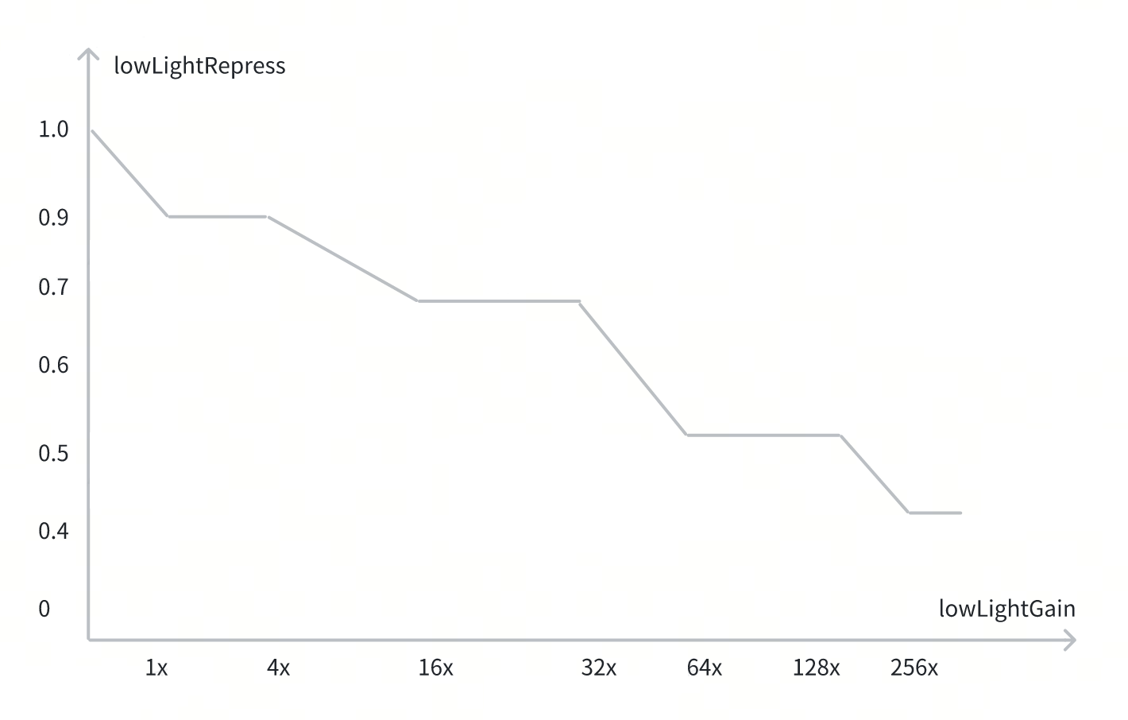
Figure 3.1‑5 Relationship between target value in low-light scenes and Gain

Damp Control

Damp Control is a function used to control the AE convergence state. By adjusting corresponding parameters, it controls the convergence speed of AE, making exposure between frames smoother. Table 3.1-5 lists parameters related to AE damping.

Parameter	Type	Range	Description	Default Value
dampOver	float	(0,1)	A value that affects the convergence speed of AE, when AE is transitioning from an overexposed state. The smaller the value, the faster the convergence.	0.7
dampUnder	float	(0,1)	A value that affects the convergence speed of AE, when AE is transitioning from an underexposed state. The smaller the value, the faster the convergence.	0.7
dampOverGain	float	(0,128)	A value that controls the exponent of the damping factor when AE is transitioning from an overexposure state. The greater the value, the faster the convergence.	1
dampUnderGain	float	(0,16)	A value that controls the exponent of the damping factor when AE is transitioning from an underexposure state. The greater the value, the faster the convergence.	1
dampOverRatio	float	(1,4)	The threshold for the AE convergence towards the target mean luminance in the overexposure direction. The greater the value, the smaller the fast convergence range. Within this threshold and the target mean luminance, the convergence is gradual.	2
dampUnderRatio	float	(0,1)	The threshold for the AE convergence towards the target mean luminance in the underexposure direction. The smaller the value, the smaller the fast convergence range. Within this threshold and the target mean luminance, the convergence is gradual.	0.5

Table 3.1‑5 AE Damping Parameters

The parameters dampOverRatio and dampOverGain are typically used to control the system’s response speed and stability. Reducing dampOver or increasing dampOverGain makes AE converge faster under bright conditions; reducing dampUnder or increasing dampUnderGain makes AE converge faster under low-light conditions. Increasing dampOverRatio reduces the fast convergence range under bright conditions; reducing dampUnderRatio reduces the fast convergence range under low-light conditions. The relationship among parameters is illustrated below.

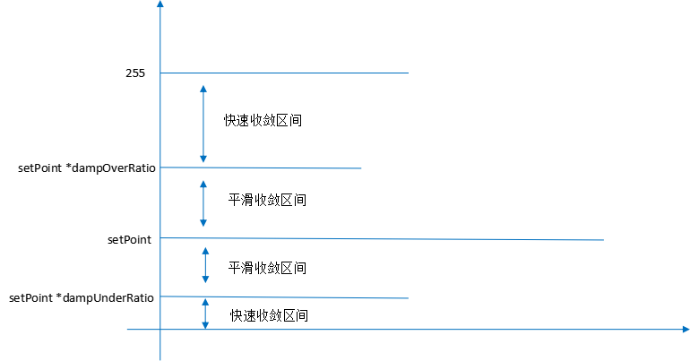
Figure 3.1‑6 AE Damp Diagram

Therefore, if fast convergence is required, it is recommended to set dampOverRatio smaller and dampOverGain larger. This configuration makes the system respond faster to changes, but care should be taken not to over-adjust, which could cause system instability. In practical applications, fine-tuning based on the system’s specific response and performance is needed to achieve optimal system performance.

Anti-Flicker

The Anti-flicker function reduces image flickering caused by artificial light sources (such as fluorescent and LED lights) by detecting the light source frequency and setting the anti-flicker mode according to the detected frequency, ensuring the camera’s exposure time synchronizes with the ambient light source frequency. Currently, anti-flicker supports the following three states:

• 50 Hz: Suitable for power frequencies in most European countries and parts of Asia.

• 60 Hz: Suitable for power frequencies in the United States and parts of the Americas.

• Custom Flicker: Users can set specific light source frequencies according to their needs. This is very useful for special environments where standard power frequencies are not 50Hz or 60Hz. Users should select the appropriate Anti-flicker setting based on their specific needs and environmental conditions. Key parameters are listed in Table 3.1‑6.

Parameter	Type	Range	Description	Default Value
antiFlickerMode	enum	AMDEV_FLIKER_PERIOD_OFF/CAMDEV_FLIKER_PERIOD_50Hz/CAMDEV_FLIKER_PERIOD_60Hz/CAMDEV_FLIKER_PERIOD_USER_DEFINED	The anti-flicker mode. Value range: l (Default) AMDEV_FLIKER_PERIOD_OFF: disable anti-flicker l CAMDEV_FLIKER_PERIOD_50Hz: the anti-flicker mode for lights whose flickering frequency is 50 Hz. l CAMDEV_FLIKER_PERIOD_60Hz: the anti-flicker mode for lights whose flickering frequency is 60 Hz. l CAMDEV_FLIKER_PERIOD_USER_DEFINED: the anti-flicker mode for user-defined light flickering frequency.	AMDEV_FLIKER_PERIOD_OFF

Table 3.1‑6 Anti-Flicker Configuration Parameters

Motion Detection

Motion detection is an important function in the auto-exposure (AE) algorithm, especially when there are drastic changes in ambient brightness or rapid camera movement, to prevent exposure jitter caused by overly rapid environmental changes. The specific process is as follows:

• When ambient brightness or camera position changes rapidly, if the system detects that the brightness change between consecutive frames exceeds a preset threshold (motionThreshold), it judges that the scene is changing rapidly, and AE enters a “lock” state, temporarily locking the current exposure settings.

• Once the environment stabilizes, AE exits the “lock” state and resumes adaptive exposure adjustment to adapt to the new ambient brightness.

Users can adjust parameters of the AE algorithm according to their needs, such as adjusting the sensitivity of exposure lock or the speed of exposure adjustment. The AE motion detection processing flow is shown in the figure below.

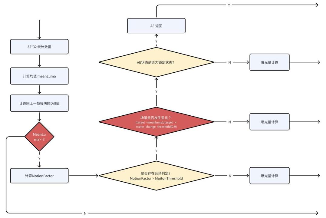
Figure 3.1‑7 AE Motion Detection Processing Flow

Key parameters for AE motion detection are listed in the table below, Table 3.1-7.

Parameter	Type	Range	Description	Default Value
motionFilter	Float	(0,1)	The damping factor when calculating motion vectors. The larger the value is, the more likely the current frame is considered to be in motion. This parameter controls the cumulative calculation of motion vectors. A greater value of motionFilter means the change of motion vectors is smoother but less timely updated. This may result in the case where the motion amplitude of the current frame is significant, but is not detected by the motion detection functionality.	0.5
motionThreshold	Float	(0,1)	The threshold for determining whether the system is in motion. When the motion vector exceeds this threshold, the current frame is considered to be in motion. This parameter determines the sensitivity of motion detection. You can reduce its value to improve the sensitivity. A more sensitive motion detection means that even slight movement of objects in the image during exposure time will be considered as motion.	0.7

Table 3.1‑7 AE Motion Detection Control Parameters

Exposure Decomposition Table

The exposure decomposition table provides exposure-related parameters, including exposure time (exposureTime), digital gain (dGain), analog gain (aGain), and image signal processing gain (ispGain). By using expDecomposeCustom and expTableNum, the exposure decomposition table can be enabled and defined, then exposure-related parameters can be obtained. The exposure time step and Gain step used in decomposing exposure are configured in the Sensor driver. Key parameters are listed in the table below.

Parameter	Type	Range	Description	Default Value
aGain	float32_t[expTableNum-1]	based on sensor limited value	Sensor analog gain array	1
dGain	float32_t[expTableNum-1]	based on sensor limited value	Sensor digital gain array	1
ispGain	float32_t[expTableNum-1]	(0,255)	ISP gain array	1
exposureTime	float32_t[expTableNum-1]	based on sensor limited value	Exposure time array.	0.01
expTableNum	uint_8	[0,8]	The number of nodes in the exposure decomposition table.	0
expDecomposeCustom	bool	{true, false}	Whether to customize exposure decomposition scheme within the sensor driver.	false

Table 3.1‑8 AE Basic Exposure Configuration Parameters

The following table illustrates the decomposition process using a lookup table. First, we define the following formula:

New exposure = exposureTime * dGain * aGain * ispDgain

The table below is an example of an exposure decomposition table.

Parameter		e0 * a0 * d0 * i0 < Exposure < e1 * a0 * d0 * i0		e1 * a0 * d0 * i0 < Exposure < e1 * a1 * d0 * i0		e1 * a1 * d0 * i0 < Exposure < e1 * a1 * d1 * i0		e1 * a1 * d1 * i0 < Exposure < e1 * a1 * d1 * i1
Exposure time	e0	Exposure / a0 * d0 * i0	e1	e1	e1	e1	e1	e1	e1
aGain	a0	a0	a0	Exposure / e1 * d0 * i0	a1	a1	a1	a1	a1
dGain	d0	d0	d0	d0	d0	Exposure / e1 * a1 * i0	d1	d1	d1
ispGain	i0	i0	i0	i0	i0	i0	i0	Exposure / e1 * a1 * d1	i1

Table 3.1‑9 AE Exposure Representation Example

The above figure shows a general exposure decomposition table. In this example, only two levels are listed for illustration; the exposure parameter decomposition patterns between all other levels follow the pattern demonstrated by these two levels. When exposure falls between two levels, exposure time is increased first, followed by aGain, dGain, and ispGain in sequence.

The actual effective exposure configuration is affected by both exposure parameters and software driver configuration. If the configured exposure table range is within the range configured by the software driver, exposure parameters will be issued according to the exposure table configuration; if the configured exposure table range exceeds the software driver configuration range, exposure parameters will be issued according to the driver configuration range, and a warning will be reported to the user side. For example, if the driver-configured exposure time range is 5ms~20ms, and the exposure table is configured with a range of 10ms~20ms, the actual effective exposure time will be issued according to the exposure table range, with a minimum exposure time of 10ms and maximum of 20ms, and no error will be reported by the software side. If the exposure table is configured with a range of 1ms~30ms, the actual effective minimum exposure time will be 5ms and maximum 20ms, and the software side will issue a warning about the exposure table exceeding limits. Gain settings are similar. It is recommended that exposure table configuration matches the software driver configuration range to avoid unexpected exposure effects.

Tuning during Phase One

In the first debugging phase, the Black Level and AWB modules need to be set to appropriate values (specific values can be referenced from detailed explanations of each module). During debugging of some front-end modules in the ISP pipeline, requirements for AE are not high, and accurate exposure values may not be necessary. For modules with low AE requirements, picture brightness can be controlled by enabling Manual AE via VTunerClient.

Fine tuning AE phase two

After completing the prerequisites listed in the table below, AE tuning can be used as the initial value for phase two of the debugging process.

Prerequisite	Status / Value
Sensor driver	Fully tested
Black level	Tuned
Lens shading	Tuned
WDR	Disabled
Initial gamma	Set
Set initial AE_LDR_Target	Objectively chosen according to the output gamma chosen

Table 3.1‑10 Prerequisites for AE Phase Two

Tuning Procedure

The tuning procedure is illustrated in Figure 3.1‑5:

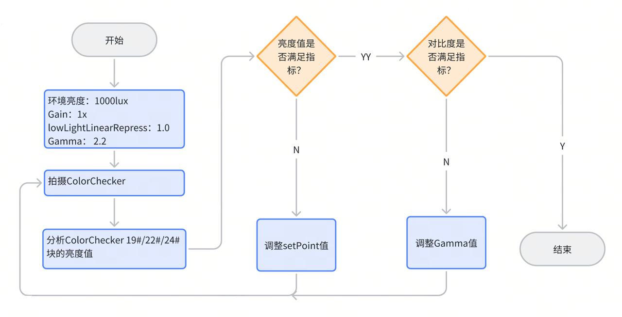
Figure 3.1‑8 Flowchart of AE Phase Two

Check the initial AE performance in a laboratory environment. Place a ColorChecker chart under 1500 lux illumination, ensuring that the ColorChecker occupies 30% ~ 50% of the image (as shown below). Capture an image and analyze the grayscale values using Imatest’s ColorChecker function, or manually analyze the grayscale patches using Adobe Photoshop or GIMP.

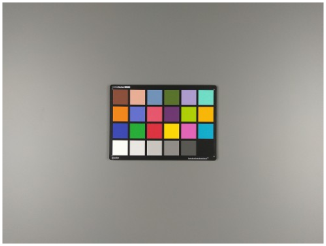
Figure 3.1‑9 ColorChecker Coverage

• Analysis using Imatest:

Imatest outputs measurement metrics such as exposure error, density response, and curve fit. f-stop values within the range of -0.25 to 0.25 are acceptable. It is recommended that the measured f-stop value falls between -0.1 and 0.

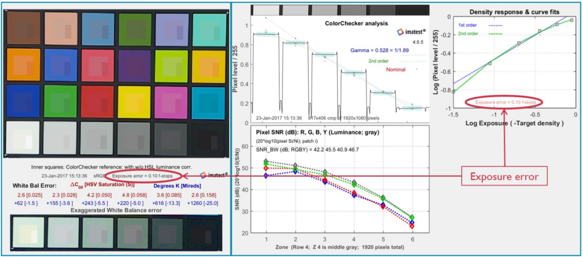
Figure 3.1‑10 Exposure Measurement Metrics

• Analysis using Photoshop or GIMP:

Use the ROI selection tool to select a portion of each gray patch on the ColorChecker. After defining the region for each patch, use the intensity/luminance histogram to calculate the mean pixel value of the selected area.

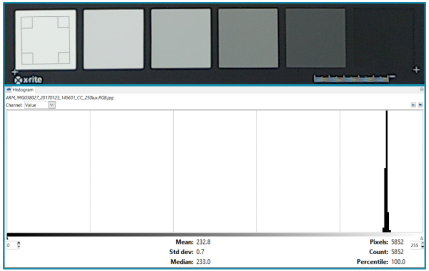
Figure 3.1‑11 Measurement of Gray Patch Pixel Mean

For an 8-bit histogram, the acceptable range of mean pixel values for each gray patch is shown in the following table. Generally, it is desirable for the measured average gray patch pixel value to be within ±10 of the ideal value. Ideally, the image should be slightly underexposed, with a deviation from the ideal value between -5 and 0.

Patch Number	Ideal Value	Minimum	Maximum
19	240	230	250
22	122	112	132
24	40	30	50

Table 3.1‑11 Recommended Values for ColorChecker Gray Patches

Note: Patch 22 represents the value of 18% gray.

The above content provides an overview of AE control and the factors influencing the AE algorithm.

Fine tuning AE phase three

Subjective Tuning in Real-Scene Laboratory Environment

After completing phase one and phase two AE tuning, subjective tuning for phase three can be conducted in a real-scene light box environment. During this phase, exposure can be increased or decreased based on requirements or preferences. The primary goal is to realistically reproduce real-world scenes and improve the subjective quality of output images. Under low-light conditions, balancing clarity and noise becomes especially critical. AE tuning should be application-driven, as the entire camera system must align with practical usage scenarios—mobile phones, surveillance, and industrial cameras each have unique requirements.

Phase three tuning mainly involves two LUTs: LowLightLinearGain and LowLightLinearRepress. These two LUTs enable dynamic adjustment of the AE target brightness under different illumination levels. The main tuning procedure is shown in Figure 3.1‑9.

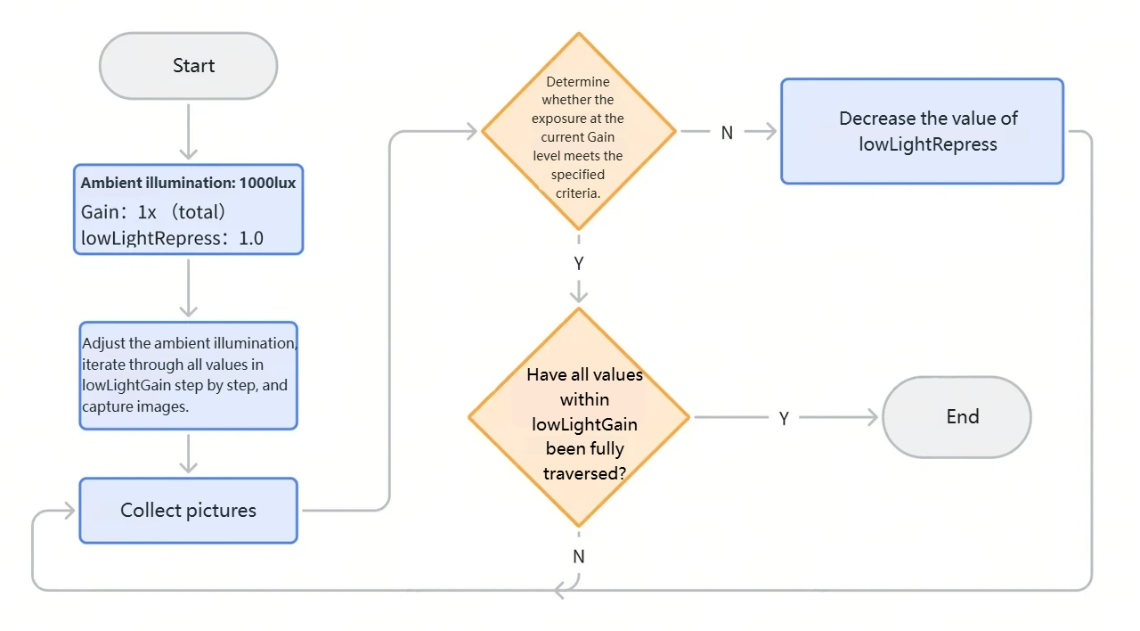
Figure 3.1‑12 AE Phase Three Tuning Flow

First, conduct validation testing in a real-scene light box. The light box should simulate real environments as closely as possible and include image test charts, objects with various colors, and different textures. Brightness can be controlled using adjustable light sources, covering a wide illumination range, typically categorized into high brightness (above 3000 lux), medium brightness (100–3000 lux), and low brightness (0–100 lux). At each brightness level, capture images and analyze the current exposure using tools from phase two (Imatest, Photoshop, and GIMP) to confirm whether the exposure falls within the acceptable range.

Seven nodes were created to define different illumination ranges, but this is insufficient. Further validation of AE performance across various illumination levels is required. For each illumination level, use Imatest/Photoshop/GIMP to analyze the luminance values of each gray patch. If values still fall outside the desired exposure range during testing, repeat the calibration steps. During optimization, it is impossible to satisfy all scenarios simultaneously, and parameter or node overlap and conflicts may occur. In such cases, trade-offs must be made based on specific requirements.

Note: When adjusting AE parameters, to avoid altering previously calibrated lookup table entries, adjustments should be made incrementally (by illumination level or gain step). In phase three, tuning should begin with the lowest system gain settings affecting all related parameters, not just the AE module. Then, incrementally increase the gain and adjust all related system parameters accordingly.

Scene Testing

After completing all laboratory tuning, final tuning must be performed in real-world environments. This helps identify differences between lab conditions and actual application environments. Before analyzing lab tuning results, capture images of diverse scenes under various lighting and weather conditions to evaluate color and texture reproduction. Use a reference camera to simultaneously capture the same scenes, enabling direct comparison between the tuned camera and the reference camera. This comparison helps identify characteristics and areas for improvement in the tuned camera.

During subjective analysis of captured images, focus particularly on areas where lab tuning failed—possibly due to poor exposure or excessive noise. Treat the reference camera’s output as the minimum acceptable quality standard, and iteratively refine previously tuned parameters until scene performance meets requirements.

Additional Tuning Information

If the image still exhibits excessive noise, consider shifting the dynamic range toward brighter regions to reduce exposure. If noise is not an issue, it is preferable to use WDR compensation and correction in dark areas while preserving highlight details.

Auto-White Balance (AWB)

Overview

Color temperature varies with the spectral composition of visible light. Under low color temperature light sources, white objects appear reddish; under high color temperature light sources, they appear bluish. The human eye uses memory-based judgment to perceive true object colors. The function of the AWB algorithm is to minimize the influence of external light sources on object color, transforming captured color information into neutral, bias-free data as if illuminated by ideal daylight.

Tuning Theory

The Auto-White Balance (AWB) module automatically adjusts the image’s white balance. AWB operates in the RAW domain. When enabled, the ISP hardware divides the frame into 32×32 blocks. The AWB algorithm calculates corresponding Rgain and Bgain values based on hardware statistics, forming a calibrated color temperature curve from the 32×32 block data. The AWB algorithm assumes the presence of “near-white” pixels in the image. It measures the distance between each block’s (R_Gain, B_Gain) and calibrated light source points. The two closest light sources are selected as primary and secondary sources. Block weights are then determined. Finally, the overall AWB gain is the weighted average of R and B gains across all blocks.

The AWB system block diagram is shown below:

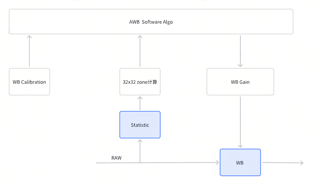
Figure 3.2‑1 AWB Processing Flow

The basic AWB tuning parameters are listed in the following table:

Parameter	Type	Range	Description	Default Value
enable	bool	{true, false}	Whether to enable AWB.	true
confidenceThreshold[10]	float32_t	[0, 3]	The radius threshold of a light source. If the distance between the (R_Gain, B_Gain) of a white block and the (R_Gain, B_Gain) of a light source exceeds this threshold, the block is assumed to be under a single light source; otherwise, it is under mixed lighting.	3 for each member
mode	enum	{CAMDEV_AWB_MODE, CAMDEV_AWB_METEDATA_MODE}	Selects the AWB mode. l CAMDEV_AWB_MODE: default AWB algorithm on the sensor. l CAMDEV_AWB_METEDATA_MODE: custom AWB algorithm on the sensor.	CAMDEV_AWB_MODE

Table 3.2‑1 Basic AWB Tuning Parameters

Statistics

The AWB Statistics module divides the entire frame into 32×32 sub-blocks and computes the average values of R, Gr, Gb, and B Bayer pixels in each block. The RAW data source can be set to one of the following: Expand, LSC, AWB Gain, or WDR.

Figure 3.2‑2 AWB Statistics Node

Solid Color Correction

Solid color correction prevents color temperature misjudgment and white balance degradation when large solid-color areas (e.g., yellow, green, blue) appear in the image. For example, when shooting a large green lawn outdoors on a sunny day, the image may appear blue because the green scene shifts the color temperature statistics toward mid-temperature ranges. To achieve accurate white balance, the ISP provides two logic methods: statistical point mapping and statistical point subtraction.

Statistical Point Mapping

The idea of statistical point mapping is to map the weights of statistical points within marked regions onto standard light sources, thereby increasing the statistical weight of standard sources in the current scene. During WB calculation, more data from standard sources will be used.

The correction process is as follows:

1. Adjust confoundPointXRg and confoundPointXBg (X = CWF/TL84/D65) to calibrate the R and B gains of green, yellow, or blue solid-color blocks under D50 illumination.

2. Enable solid color correction by setting customPositionXEnable (X = CWF/TL84/D65) to true.

3. Configure the threshold ranges for the three solid-color blocks using confoundPointXThreshold (X = CWF/TL84/D65). The threshold is the distance between a white block’s (R_Gain, B_Gain) and the center point of the solid-color block.

• A threshold that is too high may misclassify white blocks under CWF, TL84, or D65 as green, yellow, or blue blocks under D50.

• A threshold that is too low may misclassify green, yellow, or blue blocks under D50 as white blocks under CWF/TL84/D65.

  Threshold tuning should be adjusted appropriately based on the application scenario.

1. Check whether each white block falls within the calibrated blue, yellow, or green range under D50.

2. If all white blocks are within the calibrated range, change the current block’s light source to D50. Subsequent light source probability, color temperature preference, and low-light color correction will be based on the corrected D50 source.

Relevant parameters are listed in the table below.

Parameter	Type	Range	Description	Default Value
customPositionCwfEnable	bool	{true, false}	Whether to enable pure green block correction.	false
confoundPointCwfRg	float32_t	(0, 4)	The R gain of the calibrated green color block. Used to adjust the R gain calibration value of the green block under D50.	1.0
confoundPointCwfBg	float32_t	(0, 4)	The B gain of the calibrated green color block. Used to adjust the B gain calibration value of the green block under D50.	1.0
confoundPointCwfThreshold	float32_t	(0, 3)	Threshold for judging whether a block is a green block. If the (R_Gain, B_Gain) point of a block does not exceed the threshold, it is assumed to be a green block.	2.0
customPositionTl84Enable	bool	{true, false}	Whether to enable pure yellow block correction.	false
confoundPointTl84Rg	float32_t	(0, 4)	The R gain of the calibrated yellow color block. Used to adjust the R gain calibration value of the yellow block under D50.	1.0
confoundPointTl84Bg	float32_t	(0, 4)	The B gain of the calibrated yellow color block. Used to adjust the B gain calibration value of the yellow block under D50.	1.0
confoundPointTl84Threshold	float32_t	(0, 3)	Threshold for judging whether a block is a yellow block. If the (R_Gain, B_Gain) point of a block does not exceed the threshold, it is assumed to be a yellow block.	2.0
customPositionD65Enable	bool	{true, false}	Whether to enable pure blue block correction.	false
confoundPointD65Rg	float32_t	(0, 4)	The R gain of the calibrated blue color block. Used to adjust the R gain calibration value of the blue block under D50.	1.0
confoundPointD65Bg	float32_t	(0, 4)	The B gain of the calibrated blue color block. Used to adjust the B gain calibration value of the blue block under D50.	1.0
confoundPointD65Threshold	float32_t	(0, 3)	Threshold for judging whether a block is a blue block. If the (R_Gain, B_Gain) point of a block does not exceed the threshold, it is assumed to be a blue block.	2.0

Table 3.2‑2 AWB Statistical Point Mapping Parameters

Statistical Point Subtraction Function

The above statistical point mapping improves standard light source weights to correct color, but in some scenes, due to scattered statistical points or low standard source weights after mapping, white balance correction may still be incomplete. To support broader solid-color scene correction, the ISP provides a statistical point subtraction function.

This function adjusts the weights of statistical points near the location specified by confoundPositionCustom:rg/bg. Currently, up to 25 statistical regions can be subtracted. The range of each region is defined by confoundPositionCustom:threshold—the larger the value, the wider the area. The statistical weight within the region is determined by confoundPositionCustom:weight, calculated as follows:

where weight_new is the effective weight used in AWB statistics.

Correction process:

1. In a scene with color cast issues, capture a BMP/JPG image using hobotplayer.

2. Keep the shooting position unchanged, open the AWB tool in vtuner, and click the Load Image button to import the captured BMP/JPG image.

3. In the AWB tool window, click on the solid-color region in the image. The corresponding statistical point will appear on the AWB scatter plot (see yellow point in figure below). The Rgain/Bgain values of the point will be displayed on the left side of the AWB tool.

4. Set confoundPositionCustom:confoundPositionEnable to true, input the Rgain/Bgain values of the solid-color region into confoundPositionCustom:rg/bg, initially set confoundPositionCustom:weight to 0, and adjust confoundPositionCustom:threshold while observing white balance recovery. Be careful not to cover standard light source calibration points, which could affect normal scene WB. A value less than 0.5 is generally recommended. If correction is too strong, slightly increase weight or decrease threshold to normalize WB.

5. If WB is not fully corrected, subtract multiple statistical points by repeating step 4 until all necessary regions are covered.

   

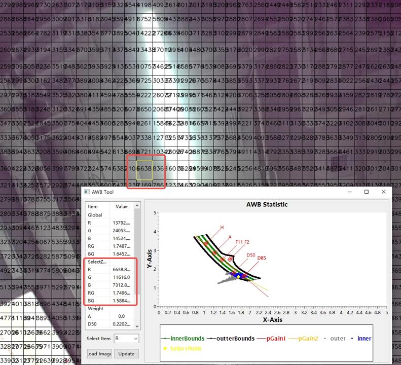
Figure 3.2‑3 Obtaining Statistical Point Data via AWB Tool

AWB point subtraction tuning parameters are listed in the following table.

Parameter	Type	Range	Description	Default Value
confoundPositionCustom:confoundPositionEnable	bool	{true, false}	Whether to enable AWB confoundPosition correction.	false
confoundPositionCustom:Index	int	[0, 24]	Index of AWB confoundPosition correction parameters	0
confoundPositionCustom:rg	float32_t	(0, 4)	Rgain center of the solid color block	1.0
confoundPositionCustom:bg	float32_t	(0, 4)	Bgain center of the solid color block	1.0
confoundPositionCustom:threshold	float32_t	(0, 3)	Range of solid color blocks.	0.3
confoundPositionCustom:weight	float32_t	[0, 1]	Degree of removal of solid color blocks. When Weight = 0, the block is completely excluded from AWB gain calculation; when Weight = 1, fully included; when Weight = 0.5, its contribution is halved compared to non-solid-color white points.	0.1

Table 3.2‑3 AWB Statistical Point Subtraction Parameters

Light Source Probability

Light source probability assigns 18 exposure levels (represented as gain multiples) to each light source (D65, D50, D75, CWF, TL84, A, or F12), stored in the 18 elements of the brightnessLevel[18] array in ascending order. Each light source has a probability at each exposure level, which affects the weight of the block’s R and B gains.

The light source order corresponds to the color temperature order during AWB calibration. To adjust the probability of a light source within a specific exposure range, first locate the corresponding group of probability parameters based on the light source order in the calibration file exported by the Calibration Tool, then modify the weight value for the desired exposure range. A higher weight increases the contribution of that light source’s (R_Gain, B_Gain) values in AWB statistics under that brightness level.

Relevant parameters are listed in the table below.

Parameter	Type	Range	Description	Default Value
lightWeightLevelEnable	bool	{true, false}	Whether to enable light source probability to adjust the weights of (R_Gain, B_Gain) values of image blocks under different light sources based on current frame brightness. Set to true to enable.	false
brightnessLevel	float[18]	[0, 17]	Exposure values of a light source. Array index represents exposure level.	1
weight	float[18]	[0, 17]	Light source probability. Increasing the j-th element (j = 0 to 17) in a light source’s weight array effectively increases the likelihood of detecting that source at brightnesslevel[j].	1

Table 3.2‑4 Light Source Probability Parameters

Color Correction

Color correction is used to correct color bias in low-light conditions.

The light source probability parameters provide 18 exposure levels for each light source (D65, D50, D75, CWF, TL84, A, or F12), expressed as gain multiples. Exposure amount and R/B channel gains are configured via brightnessLevel, grayRgain, and grayBgain, with brightnessLevel in ascending order. Based on environmental conditions, the exposure level and primary light source are determined, and the required R and B gains for white blocks under the primary source are interpolated from grayBgain and grayRgain.

The light source order corresponds to the color temperature order during AWB calibration. To adjust color correction for a specific light source within a certain exposure range, first locate the corresponding parameter group based on the AWB module’s light source order in the calibration file, then modify grayRgain and grayBgain for the desired exposure range to achieve color adjustments at different exposure levels.

The following table provides detailed information on color correction parameters.

Parameter	Type	Range	Description	Default Value
preferenceGainEnable	bool	{true, false}	Whether to enable color correction to correct bias caused by different light intensities. Set to true to enable.	false
brightnessLevel	float[18]	[0, 17]	Exposure value of a light source. Array index represents exposure level. Higher exposure amount indicates lower environmental brightness.	1
grayBgain	float[18]	(0, 512)	Gains of the blue channel relative to 256. Array index represents exposure level.	256
grayRgain	float[18]	(0, 512)	Gains of the red channel relative to 256. Array index represents exposure level.	256
useCcoffset	bool	{true, false}	Whether to add offsets to the color correction matrix (CCM).	true
useCcmatrix	bool	{true, false}	Whether to use CCM for further color correction.	true

Table 3.2‑5 Color Correction Parameters

Color Temperature Preference

Color temperature preference allows adjustment of image tone toward red/yellow or blue/purple under different color temperatures while maintaining overall well-tuned AWB. After identifying the ambient color temperature, the preference gain multiplies the original R and B gain values. This color preference adjustment is solely related to ambient color temperature, not exposure. For fine-tuning involving exposure, use the color correction function in Section 3.2.2.4.

Relevant parameters are listed below.

Parameter	Type	Range	Description	Default Value
temperatureEnable	bool	{true, false}	Whether to enable color temperature preference. Set to true to enable.	false
preferenceA	uint16_t	(0, 512)	Color preference for low-temperature light, implemented by modifying R gain. Increasing the value results in a redder image under light A.	256
preferenceCwf	uint16_t	(0, 512)	Color preference for mid-temperature light, implemented by modifying R gain under CWF. Increasing the value results in a redder image.	256
preferenceD65	uint16_t	(0, 512)	Color preference for high-temperature light, implemented by modifying B gain. Increasing the value results in a bluer image under D65.	256

Table 3.2‑6 Color Temperature Preference Parameters

Face AWB

Face AWB works as follows:

1. Obtain R and B gain values from the ROI of the face area.

2. Adjust the obtained R and B gains based on face color preference.

3. Compute the average of the adjusted R and B gains to obtain average gains for the face region.

4. Weight the average R and B gains of the face region to compute the overall image R and B gains.

Face AWB parameters are listed below.

Parameter	Type	Range	Description	Default Value
faceAwbEnable	bool	{true, false}	Whether to enable face AWB. Must be set to true to enable.	false
faceAwbRoiNum	uint8_t	[0, 1]	Number of face ROIs.	0
faceWeight	uint32_t	[0, 1]	Proportion of face AWB in overall AWB gain calculation. Higher values increase the impact of face AWB gains on the entire image, resulting in a more purplish image (because face R and B gains are higher than white blocks).	0.5
faceAwbRg	uint32_t	(0, 256)	Preference for R gain in face AWB. Higher values make the face and entire image redder after AWB processing.	256
faceAwbBg	uint32_t	(0, 256)	Preference for B gain in face AWB. Higher values make the face and entire image bluer after AWB processing.	256

Table 3.2‑7 Face AWB Parameters

ROI AWB

ROI AWB works as follows:

1. Obtain R and B gain values from the ROI.

2. Compute the average of the obtained R and B gains to get average gains for the ROI.

3. Weight the average R and B gains to obtain the overall AWB gain.

Detailed ROI AWB parameters are listed below.

Parameter	Type	Range	Description	Default Value
roiNumber	uint8_t	[0, 25]	Number of ROI regions for ROI AWB. Must be greater than 0 to enable.	0
roiWeight	float32_t	[0, 1]	Weight of the AWB gain calculated by ROI AWB in the overall AWB gain. Higher values increase the impact of ROI AWB gains.	0.5
roiWindow	Vsi3ARoiWindow_t[25*5] where Vsi3ARoiWindow_t{ float32_t fx; float32_t fy; float32_t fw; float32_t fh; float32_t weight}	Weight: [0, 255]; others depend on image size	ROI window information: l fx: horizontal start. l fy: vertical start. l fw: width. l fh: height. l weight: ROI weight.	[0,0,100,100,1]

Table 3.2‑8 ROI AWB Parameters

AWB Damp Control

To avoid AWB fluctuations caused by sudden exposure changes (e.g., moving from a dark room to bright outdoor), AWB must respond quickly when exposure changes significantly, but remain stable when changes are minor. AWB damping smooths transitions to avoid overshoot or jitter. Higher damping results in slower but more stable convergence. AWB convergence can be controlled via the AWB damping coefficient.

Parameter	Type	Range	Description	Default Value
useDamping	bool	{true, false}	Whether to enable damping. Must be set to true to enable AWB damping.	true
useManuDampCoeff	bool	{true, false}	Whether to set the damping coefficient manually. If false, AWB automatically calculates manuDampCoeff based on exposure variation.	false
manuDampCoeff	float	(0, 1)	AWB damping coefficient. Higher values result in smoother convergence, reducing color changes between frames.	0.5

Table 3.2‑9 AWB Damping Control Parameters

White balance correction for each channel is completed by AWB statistics and algorithms based on static calibration results. This correction is not updated in frame data but is applied as part of the configuration in the next frame.

AWB Locking and Unlocking

Changes in ambient color temperature may affect the AWB lock state.

Table 3.2‑11 lists parameters for adjusting AWB lock thresholds. Once the threshold exceeds 0, the AWB lock function is enabled. Values that are too high or too low may cause the AWB to remain locked or unlocked, leading to inaccurate image colors after AWB processing.

Parameter	Type	Range	Description	Default Value
awbEnterUnlockThreshold	float32_t	[0, 0.2]	Threshold for AWB to enter unlocked state. Higher values make it harder for AWB to lock.	0
awbEnterLockThreshold	float32_t	[0, 0.2]	Threshold for AWB to enter locked state. Higher values make it easier for AWB to lock.	0

Table 3.2‑10 AWB Lock/Unlock Parameters

Tuning during phase one

Pre-tuning Preparation

Parameter name	Description
Black level	Tuned
Lens shading	Tuned
CCM	Tuned
GAMMA	Tuned
Manual exposure	-0.25 < exposure error < 0.25 (f-stops). Can be verified via Imatest.

Table 3.2‑11 AWB Phase One Preparation Conditions

Calibration images

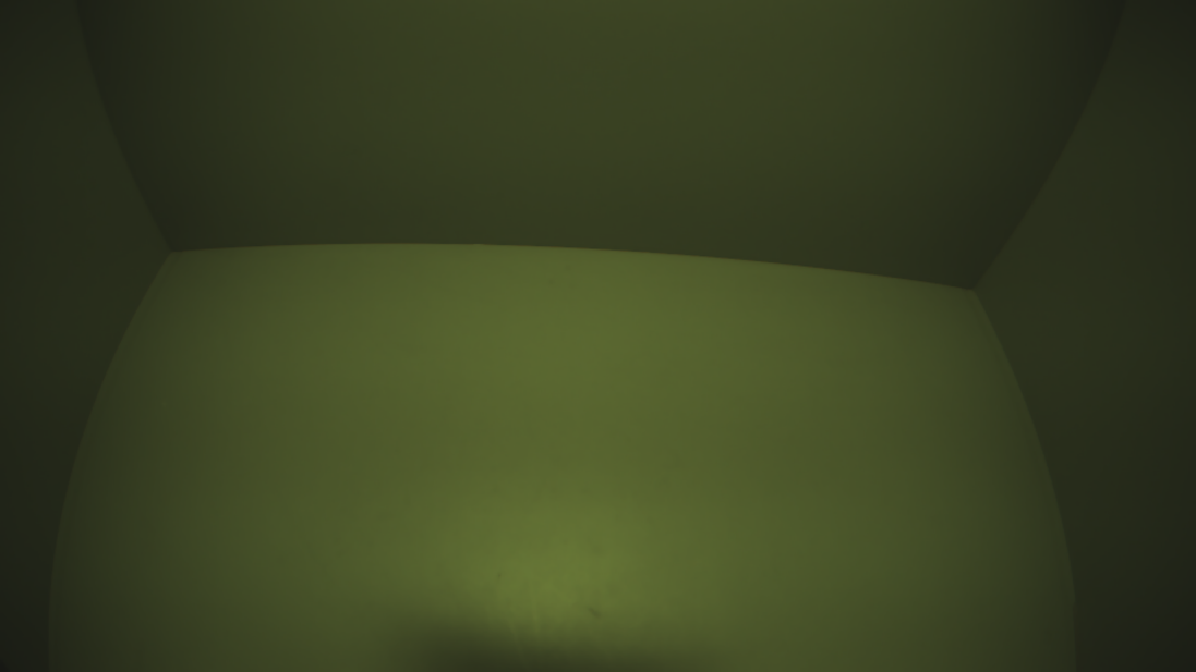
Figure 3.2‑4 AWB Calibration Backboard Image

The CalibrationTool is used to collect RAW data of ColorChecker and light box walls under standard light boxes with different color temperatures for WB calibration. Refer to the “X5-Calibration Tool User Guide” for detailed calibration procedures. Calibration calculations on RAW images at different color temperatures are used to calibrate the Planckian curve.

Capture RAW data of gray cards or light box walls under as many color temperatures as possible, as listed in the table below. D50 and CWF sources are essential, and at least five light sources should be included to ensure algorithm coverage across more scenes.

Note: Use a color meter (e.g., Minolta CL-200A) to record color temperature values when capturing RAW data.

Illuminant	Color Temperature	Planckian/non-Planckian
10K	10000K	Planckian
D75	7500K	Planckian
D65	6500K	Planckian
D50	5000K	Planckian
CWF	4150K	Non-Planckian (Extra)
D40	4000K	Planckian
TL84	3800K	Planckian
TL83	2800K	Planckian
A	2800K	Planckian
H	2300K	Planckian

Table 3.2‑12 AWB Calibration Color Temperature List

When performing Planckian curve-based calibration, several key points must be observed to ensure accuracy, especially when selecting white regions:

1. White Region Selection: In the Calibration Tool, manually drag the selection box to include all captured gray card points, which are critical reference points for calibration. Avoid making the box too large to prevent including irrelevant areas that could affect AWB accuracy.

2. Distance Control: The box should tightly surround the gray card points without being too far. An oversized box may capture extraneous color information, leading to inaccurate AWB.

3. Calibration Processing: When calibrating collected RAW data, ensure that RAW data is processed through the Lens Shading Correction module in the CalibrationTool to subtract BLS and LSC. If LSC is not applied, the loaded LSC configuration will be zero.

Tuning verification using Imatest

Run the ColorChecker image using the Colorcheck option in Imatest. This generates a series of color charts for analysis. Extract the HSV (Hue, Saturation, Value) of patches 20–22 and compute their average.

Additionally, refer to the numerical values to assess AWB performance. Final results depend on image sensor quality and customer requirements.

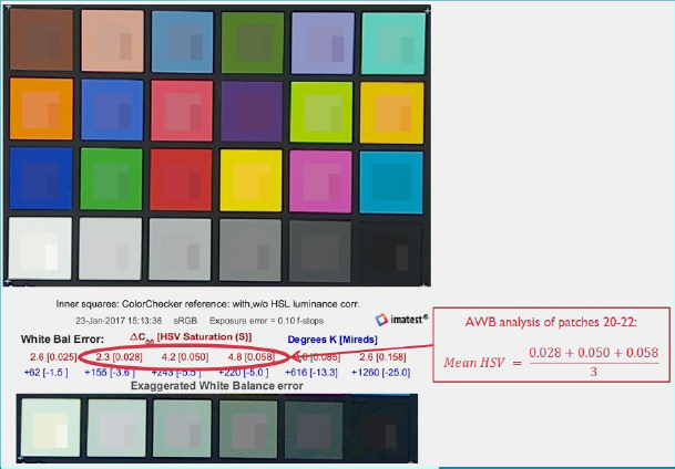
Figure 3.2‑5 Imatest Color Analysis Window

AWB quality	6,500K (HSV)	4,000K (HSV)	2,700K (HSV)
Great	<0.025	<0.035	<0.030
Good	0.025–0.050	0.035–0.060	0.030–0.065
Fair	0.050–0.100	0.060–0.110	0.065–0.160
Poor	>0.100	>0.110	>0.160

Table 3.2‑13 AWB HSV Data Reference

Fine tuning AWB phase three

Adjust other configurable AWB parameters in phase three.

Tuning color preference model

During gain compensation, the AWB algorithm generates a gain value for each color channel to render gray objects as neutral gray. Before final AWB application, the preference gain module can adjust the final compensation gains to achieve better or subjectively preferred color tints. Each channel uses an 8-bit precision gain value, and three CCT values are used to divide the color temperature range. Default gain is 256 for all color temperatures.

Temperature Weight

In AWB parameter configuration, custom weights can be assigned to different color temperatures. The figure below shows an example of weight settings.

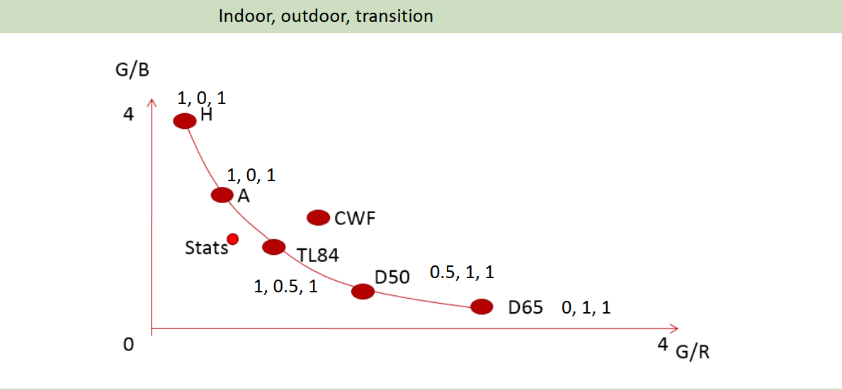
Figure 3.2‑6 AWB Color Temperature Weight Settings

AWB verify

Refer to the “VTunerTool User Manual” for instructions on verifying image white balance performance using calibrated AWB data.

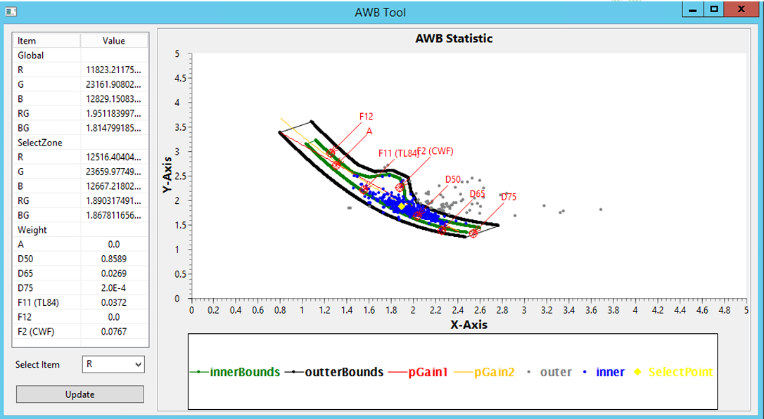
Figure 3.2‑7 AWB Verify Example

High Dynamic Range (DOL2)

Overview

The dynamic range of real-world scenes far exceeds the usable dynamic range of low-cost CMOS image sensors. Therefore, image sensors capture a limited range (LDR) and map it to their available output range. Radiance levels above or below this sensor range are clipped to black or white.

HDR combines two frames with different exposures into a single frame. The resulting single frame has higher precision than either original frame. Fundamentally, this algorithm uses short exposure to preserve highlight details and long exposure to retain shadow details without excessive noise, thereby increasing the camera system’s dynamic range.

The HDR module stitches two 12/16-bit frames into a 20-bit frame without accessing DDR, capturing more image information (bright and dark areas). The WDR module then reduces the enhanced 20-bit frame back to 12 bits, preserving more content than the original linear frame. The exposure ratio between frames is determined by exposure time and gain. For DOL2 mode, all exposures can be aligned to short-exposure saturation or long-exposure alignment.

The HDR module includes the following sub-functions:

• Pre-Process Module (BLS, AWB, DG)

• Histogram Statistics

• Combine Module

• Deghost

Tuning theory

The main basic algorithm flow of the HDR module: In dual-frame HDR, the long and short frames undergo preprocessing, followed by motion detection, and finally are combined into a high dynamic range image. The preprocessing stage includes several modules—mainly BLC, DGain (detail gain), and AWB—which compute the image’s grayscale luminance. After motion detection for deghosting, the frames are merged into a high dynamic range image.

The overall DOL2 processing flow is shown below:

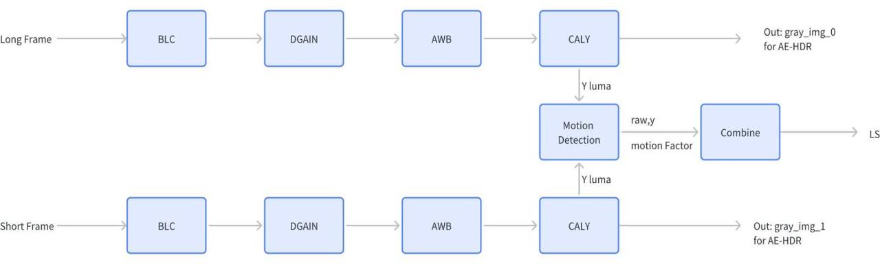
Figure 3.3‑1 HDR Processing Flow

BLC

The BLC module in HDR preprocessing allows separate setting of BLC values for four channels in different exposure frames.

The following table lists the HDR preprocessing BLS parameters.

Parameter	Type	Range	Description	Default Value
bls[4]	int	[0,4095]	BLS values in R, Gr, Gb, and B channels.	[0,0,0,0]

Table 3.3‑1 HDR BLS Configuration Parameters

Digital Gain

The Dgain module in HDR preprocessing allows separate setting of Dgain values for four channels in different exposure frames, used to enhance RAW image brightness. The following table lists HDR preprocessing parameters.

Parameter	Type	Range	Description	Default Value
dgainEnable	bool	{true, false}	true: enables digital gain; false: disables it.	[0,0,0,0]
dgain	Float[4][4]	/	Digital gains in the format: [[l_r, l_b, l_gr, l_gb], [s_r, s_b, s_gr, s_gb], [vs_r, vs_b, vs_gr, vs_gb], [e3_r, e3_b, e3_gr, e3_gb]].	[[1.0, 1.0, 1.0, 1.0], [1.0, 1.0, 1.0, 1.0], [1.0, 1.0, 1.0, 1.0], [1.0, 1.0, 1.0, 1.0]]

Table 3.3‑2 HDR DGain Configuration Parameters

Combine Module

In HDR Stitch linear mode, the long exposure frame can be combined into the short exposure frame, or vice versa.

For example, a base frame is called Fbase, and an exposure frame to be combined is called Fin. Fbase and Fin are combined using a weighting factor W and exposure ratio R, calculated as follows:

In dual-frame HDR fusion, two different combination modes exist, reflected in two different configurations in actual combine parameters.

Linear Combination

In linear mode, the longer exposure can be merged into the shorter one, or vice versa. For convenience, assume the base frame is B and the exposure frame to be merged is E. Two important parameters affect the result: ratio and transmission range. If Deghost is enabled, Motion_factor is added. The ratio multiplies E; if B is the shorter frame, the ratio is less than 1 (represented as 12-bit fractional). Otherwise, it is an 8-bit integer with 4-bit fractional part.

Non-linear Combination

Used when merging short exposure into long exposure data, especially when there is a large sensitivity gap. Short exposure noise is high, and saturation levels cannot be mixed on a linear scale.

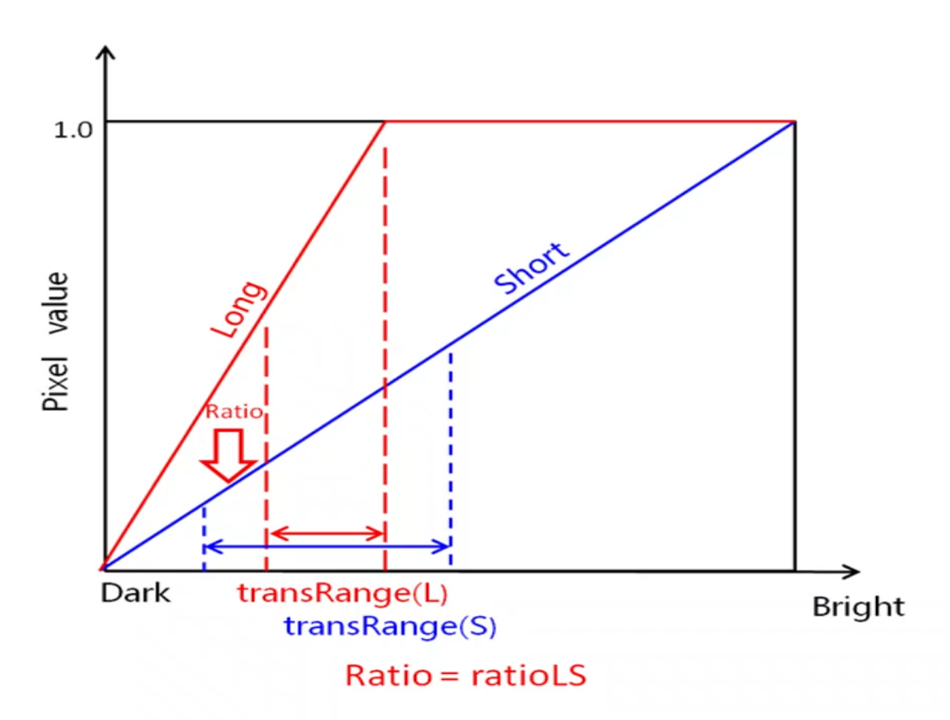
Figure 3.3‑2 HDR Combine Processing Illustration

The following table explains HDR Combine parameters.

Parameter	Type	Range	Description	Default Value
bypassSelect	int	[0,2]	0: outputs only long frames. 1: outputs only short frames. 2: outputs only very short frames.	0
colorWeight	int[3]	[0,255]	The color weights, in format [stitchColorWeight0, stitchColorWeight1, stitchColorWeight2] where: l stitchColorWeight0: the weight for the channel with the greatest value l stitchColorWeight1: the weight for the channels with in-between values l stitchColorWeight2: the weight for the channel with the smallest value The weights must meet the following requirement:stitchColorWeight0 + stitchColorWeight1× 2+ stitchColorWeight2= 256 The greater the stitchColorWeight0, the easier it is to combine short frames at the saturation point of the corresponding channel. If the short-frame noise is very large, stitchColorWeight0 can be reduced and the other weights can be increased. For noise reduction, this parameter has a lower priority than transRange.	[255,0,1]
stitchingMode	int	[0,1]	0: linear stitching mode. 1: non-linear stitching mode.	0
baseFrame	int	[0,1]	0: based on S frames. 1: based on L frames.	0
ratio	float[2]	[1.0,256.0]	The exposure ratios, in the following format: [long/short, short/very short].	[16.0,16.0]
transRange	float[4][2]	[0.0,1.1]	The start and end values of each composite interval, where two frames overlap. The value must be in the following format: [[L+S_ref(L)_start, L+S_ref(L)_end], [LS+VS_ref(LS)_start, LS+VS_ref(LS)_end],[L+S_ref(S)_start, L+S+ref(S)_end],[LS+VS_ref(VS)_start, LS+VS_ref(VS)_end]]. If the pixels of the reference frame are lower than the start value, the composite frame pixels are longer frames. If the pixels of the reference frame are higher than the end value, the composite frame pixels are short frames. If the pixels of the reference frame are within the interval, the composite frame pixels are a fusion of the long and short frames.	[[0.2, 0.9], [0.0, 0.9], [0.95, 1.0], [0, 0.1]]

Table 3.3‑3 HDR Combine Parameter Description

Deghost Module

Since short-exposure and long-exposure frames are captured at different times, ghosting artifacts may appear in the merged image if there are moving objects in the scene. Therefore, a motion detection function is added. The motion detection should identify moving regions and replace them with short-exposure images. Because the sensor is linear, L should equal ratioLS*S; otherwise, motion artifacts may occur. The pixel motion degree is marked by Motion_factor and used in multi-exposure merging calculations.

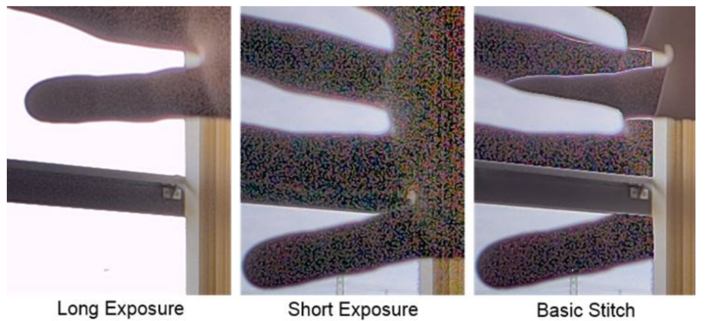
Figure 3.3‑3 Example of Motion Artifacts

The Deghost module adjusts the lower threshold and the lower threshold for dark regions based on the relationship between motionValue and motionFactor.

Parameter	Type	Range	Description	Default Value
extentBit	Int[2]	[-1,8]	The value of the extended bits, in format [L/S merge, LS/VS merge]. 0 to 8: The extended bits are set to the specified value. -1: (Recommended) The extend bit is automatically calculated according to the ratio.	[-1,1]
motionEnable	bool[2]	{true, false}	true: enables deghost. false: disables deghost.	[false, false]
motionWeight	int[2]	[0, 1024]	The weights of the moving area.	[0,0]
motionWeightShorter	int	[0, 1024]	The weight of shorter frames in the moving area.	473
motionSatThreshold	int	[0, 1024]	The saturation threshold for motion detection.	4096
motionWeightUpdateThreshold	int	[0,8191]	The weight update threshold.	1024
motionLowerThresholdLs	int[4]	[0,2047]	The motion detection thresholds in [gr, r, b, gb] order. It is recommended to increase the parameter values as the shorter-frame gain increases.	[16,16,16,16]
motionLowerThresholdLsvs	int[4]	[0, 4095]	The motion detection thresholds in [gr, r, b, gb] order. It is recommended to increase the parameter values as the shorter-frame gain increases.	[16,16,16,16]
motionUpperThresholdLs	int[4]	[0, 4095]	The motion detection thresholds in [gr, r, b, gb] order. It is recommended to increase the parameter values as the shorter-frame gain increases.	[120,120,120,120]
motionUpperThresholdLsvs	int[4]	[0, 4095]	The motion detection thresholds in [gr, r, b, gb] order. It is recommended to increase the parameter values as the shorter-frame gain increases.	[120,120,120,120]
darkLowerThresholdLs	int[4]	[0, 4095]	The dark area thresholds in [gr, r, b, gb] order. It is recommended to increase the parameter values as the shorter-frame gain increases.	[16,16,16,16]
darkLowerThresholdLsvs	int[4]	[0, 4095]	The dark area thresholds in [gr, r, b, gb] order. It is recommended to increase the parameter values as the shorter-frame gain increases.	[16,16,16,16]
darkUpperThresholdLs	int[4]	[0, 4095]	The dark area thresholds in [gr, r, b, gb] order. It is recommended to increase the parameter values as the shorter-frame gain increases.	[256,256,256,256]
darkUpperThresholdLsvs	int[4]	[0, 4095]	The dark area thresholds in [gr, r, b, gb] order. It is recommended to increase the parameter values as the shorter-frame gain increases.	[256,256,256,256]
dpfLConfig.div	float	[1.0, 64.0]	The division factor. A greater value leads to less denoise strength.	0

Table 3.3‑4 HDR Deghost Tuning Parameters

MotionDetection

The motion detection assumption is based on a linear sensor. The long frame should satisfy the criterion of ratio * short frame; otherwise, motion may exist. In the algorithm, a motion value is calculated as the difference between the long frame and ratio * short frame. Then, a normalized range defined by motion lower threshold and motion upper threshold is used to compute the motion factor, which estimates whether motion exists.

There are two criteria for determining motion:

1. Threshold-based detection. Below the lower threshold, the value is set to 0; above the upper threshold, it is set to 1024. Areas below thr_low are considered static; areas above thr_high are considered moving.

2. Replacement for dark regions. Some areas in the short frame may be too dark, causing deviations from the linear relationship in static regions. Or, the brightness values in very dark areas are too low to provide useful information, so even if a region is moving, short-exposure data cannot be used to replace it.

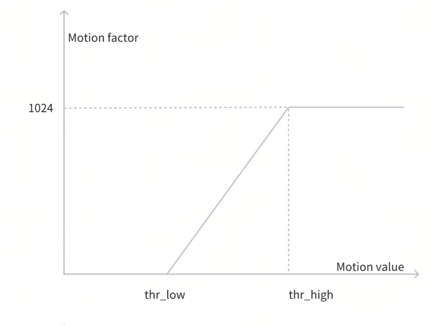
Figure 3.3‑4 Motion Factor Curve

Compand

Overview

The Compand module performs data compression and decompression, consisting of two sub-modules: expand and compress. The Expand sub-module extends input data (12–20 bits) to 20-bit raw data; the Compress sub-module compresses 20-bit raw data into output data (12–20 bits).

Tuning Theory

In the Expand Curve, X and Y represent the nodes of the input-output curve. Internally, these values are stored in two RAM tables, one for X and one for Y, each containing 64 entries. Each memory row can be individually addressed via the ISP_COMPAND_EXPAND_x_ADDR register, and its value can be read or written using the ISP_COMPAND_EXPAND_x_WRITE_DATA register. The table below shows example curve parameters for the compand module.

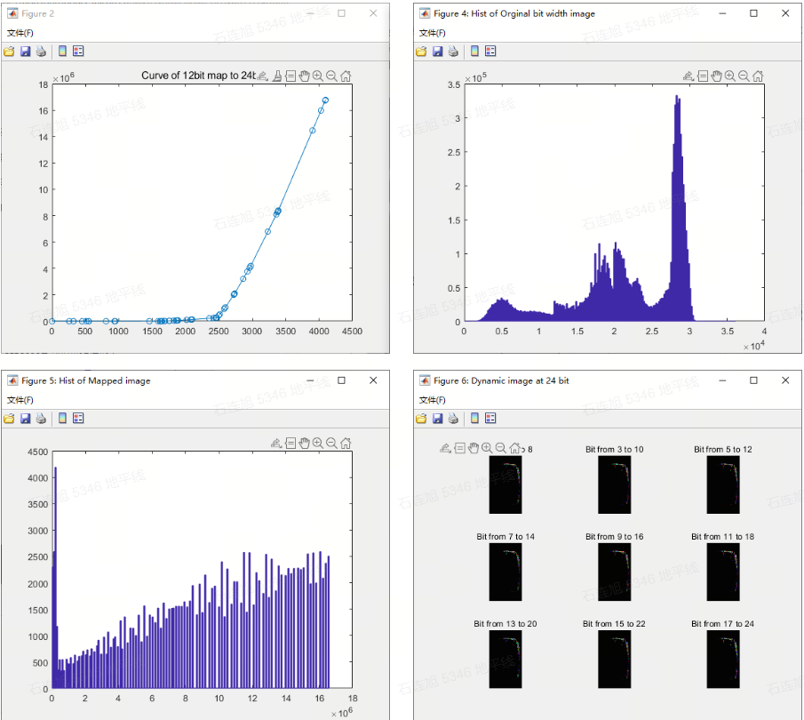
Figure 3.4‑1 Compand Module Curve Diagram

Relevant tuning parameters are as follows:

Parameter	Type	Range	Description	Default Value
expandEnable	bool	{true, false}	Enable expand in the compand module	false
expandCurveX[64]	int[64]	[0,24]	x stands for the distance in expand curve Distance_n = 1 << expand_px_n	-
expandCurveY[64]	int[64]	[0, 1048576]	y stands for the value	-
expandUseOutYCurve	bool	{true, false}	false: Use the built-in fixed formula to calculate y using the configured x true: Use the manual configured y value	false
compressEnable	bool	{true, false}	Enable compress in the compand module	false
compress CurveX[64]	int[64]	[0,24]	x stands for the distance in expand curve Distance_n = 1 << compress_px_n	[20, 18, 14, 20, 18, 14, 20, 18, 14, 13, 20, 18, 14,20, 18, 14, 13, 20, 18, 14, 20, 18, 14, 13, 20, 18,14, 13, 15]
compress CurveY[64]	int[64]	[0, 1048576]	y stands for the value	[ 8192, 14640, 16256, 16352, 29232, 32464, 32672, 32768, 58576, 65024, 65440, 65744, 117360, 130272, 131072, 234320, 260128, 261744, 467824, 519456, 522672, 524288, 937264, 1040512, 1046960, 1871312, 2077792, 2090704, 2097152, 3749056, 4162048, 4187856, 7485216, 8311168, 8362800, 8388608, 14996256, 16648160, 16751408, 16777216, 16777216 ]
compressUseOutYCurve	bool	{true, false}	false: Use the built-in fixed formula to calculate y using the configured x true: Use the manual configured y value	false

Table 3.4‑1 Expand Tuning Parameters

Expand Phase One Tuning

Follow the corresponding section in the “X5-Calibration Tool User Guide” document to calibrate parameters and obtain the parameter values for the Expand module.

Black Level Subtraction

Overview

Black Level Subtraction is the first module in the pipeline that requires tuning, and all other modules depend on black level correction. Therefore, it is one of the most fundamental modules and is rarely re-adjusted after initial calibration. The tuning process is as follows:

• Phase One: Calibrate black level values at different gains using the Calibration Tool.

• Phase Two: No tuning required unless previous calibration results are poor.

• Phase Three: No tuning required unless previous calibration results are poor or uncalibrated lighting conditions are encountered in real-world scenarios.

Tuning Theory

The image sensor’s black level varies with temperature, analog gain, and exposure time. Most sensor manufacturers do not provide temperature-related information. Therefore, in the ISP, black level is only associated with analog gain. The BLS module parameters are included in the VTunerClient under Black Level Subtraction.

Parameter	Type	Range	Description	Default Value
bls[4]	int	[0,4095]	BLS values in R, Gr, Gb, and B channels.	[0,0,0,0]

Table 3.5‑1 BLC Parameters

Black Level Phase One Tuning

Follow the corresponding section in the “X5-Calibration Tool User Guide” document to calibrate parameters and obtain the black level values for the four channels at different gains.

RGB Infrared Radiation

Overview

The RGBIR module processes 4x4 RGBIR data patterns. It converts RGBIR data into RGB Bayer data and IR data for subsequent ISP pipeline processing.

The tuning process is as follows:

• Phase One: Use VTunerClient to calibrate the IR component.

• Phase Two: Adjust the IR component subtraction ratio in highlight regions.

• Phase Three: Adjust backend ISP pipeline module parameters, using the same method as for RGGB pattern mode.

Tuning Theory

Traditional CMOS image sensors use the Bayer pattern as the color filter array (CFA). Pixel color information is determined by specific wavelengths of light. RGB-IR technology uses an RGB-IR CFA, modifying some pixels in the Bayer format to IR pixels that only allow infrared light to pass through.

When processing RGB-IR data, the 4x4 RGBIR pattern must be restored to RGGB pattern, and the IR channel must be extracted for subsequent processing. The internal processing of the RGBIR module functions like a small pipeline, including the following functions:

• Pattern normalization

• Black level subtraction (BLS)

• DPCC RGBIR (defect pixel correction)

• Denoise and upscale IR channel to full resolution

• Interpolate G channel to full resolution

• Interpolate B&R channels at R&B&G positions

• Remove IR component

• Downsample to RGB Bayer

• Revert to normal RGB

The RGBIR pipeline can be represented as shown in Figure 3.6‑1.

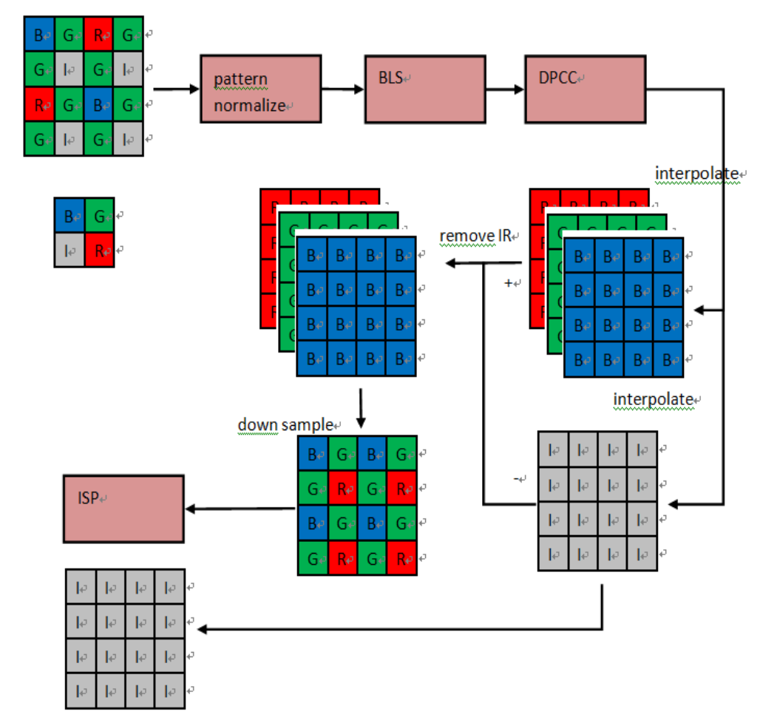
Figure 3.6‑1 RGBIR Processing Flowchart

The parameters used for RGBIR pattern tuning are listed below.

Parameter	Type	Range	Description	Default Value
enable	bool	{true, false}	Enable the RGBIR module.	false
irThreshold	int	[0,4095]	Infrared channel de-saturation curve.	4095
lThreshold	int	[0,4095]	Remove IR. When light > I_threshold_start, the weight curve drops, gets smaller. When light > I_threshold_end, weight = 0	4095
dpccTh[4]	Int[4]	[0, 65535]	DPCC abs(center_pixel - avg) > th as defect point, 0~4095, 4095 as not DPCC	[4095, 4095,4095, 4095]
dpccMidTh[4]	Int[4]	[0, 65535]	FFF000	[4095, 4095,4095, 4095]
ccMatrix[12]	float[12]	[-4.0, 4.0]	3*4 color conversion matrix	[1.0, 0.0, 0.0, 0.0, 0.0, 1.0, 0.0, 0.0, 0.0, 0.0, 1.0, 0.0]
gain[3]	float[3]	[0.0, 4.0]	WB gain	[1.0, 1.0, 1.0]

Table 3.6‑1 RGBIR Tuning Parameters

RGBIR BLS

Black level compensation is a process of subtracting calibrated black level offset values to correct baseline variations in the image or signal.

Parameter	Type	Range	Description	Default Value
bls[4]	int	[0,4095]	BLS values in R, Gr, Gb, and B channels.	[0,0,0,0]

Table 3.6‑2 RGBIR BLC Tuning Parameters

RGBIR DPCC

DPCC is applied after the RGBIR module. Since defective pixels in the RGBIR module may spread due to interpolation, the RGBIR module must include a DPCC module to correct these defects.

The DPCC module includes two sets of parameters: Dpcc_threshold and Dpcc_median_threshold, as explained in Table 3.6‑1. These parameters must be adjusted based on the characteristics of defective pixels. If set too low, they may damage the image.

RGBIR Remove IR

Since each channel in an RGBIR sensor contains an infrared (IR) component, the IR component must be subtracted from each channel to restore normal RGB.

The values of a 3x4 matrix are determined by the sensor’s spectral response curve. Typically, the following matrix is used, where the first three columns form an identity matrix, and the last column is -1, used to define the proportion of IR component subtraction from the R/G/B channels.

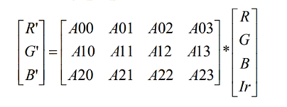
Figure 3.6‑2 RGBIR IR Removal Processing Matrix

For example, the calculation for removing the IR component from the original R channel is:

The last column of the 3x4 matrix determines the IR subtraction ratio. Different subtraction ratios result in different visual effects, as shown in Figure 3.6‑3.

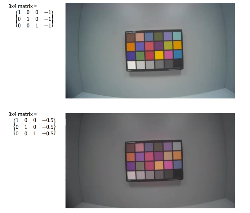
Figure 3.6‑3 RGBIR IR Removal Comparison with Different Configurations

Highlight IR Desaturation

When processing color-saturated regions, such as skies or highlights, directly applying the original matrix may cause color shifts because the changes in each color channel in saturated regions are not linear.

By setting thresholds Th_l and Th_h, the system determines whether the current region is oversaturated based on brightness. The IR coefficients in the R/G/B channels of the matrix are adjusted to reduce the proportion of IR component removal, thereby weakening the IR value and avoiding issues caused by oversaturation.

The processing flow for saturated and transition regions is as follows:

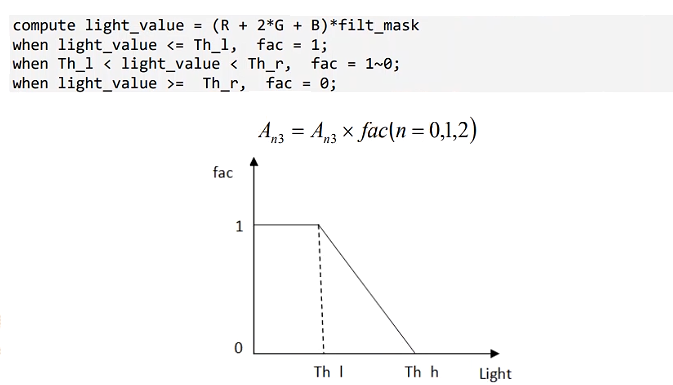
Figure 3.6‑4 RGBIR Highlight Processing Flowchart

Lens Shading Correction

Overview

Shading refers to the vignetting effect caused by uneven brightness between the center and periphery of the lens image. The Lens Shading module corrects this issue. It also corrects chroma shading (color uniformity), which is critical for accurate color reproduction.

Shading characteristics are related to module properties, depending on the manufacturer’s optical assembly process and IR filter performance. Additionally, different lighting conditions affect chroma shading, and sometimes Ir cut filters fail to provide accurate wavelength cutoffs, causing issues.

The module tuning overview is as follows:

• Phase One: Calibrate Lens Shading under standard laboratory lighting using the Calibration Tool.

• Phase Two: No adjustment needed unless other modules cause shading correction issues.

• Phase Three: No adjustment needed unless other modules cause shading correction issues or uncalibrated lighting conditions are encountered in real-world applications.

Tuning Theory

The LSC module corrects spatial or asymmetric shading distortions by mapping corrections across the entire image. The shading correction data includes correction values for all four Bayer channels. The goal of the shading correction algorithm is to achieve uniform brightness and color across the entire image. Thus, each input pixel PIN(x, y) is multiplied by a correction factor F(x, y). The correction factor is a fixed-point number with 4 integer bits and 10 fractional bits, effective range [1.0, 15.999]. The correction factor depends on the pixel’s coordinates and color.

The corrected pixel value PCOR(x, y) is calculated as:

To improve correction accuracy, the image is divided into 32 regions in both x and y dimensions. The figure below illustrates the lens shading correction region layout.

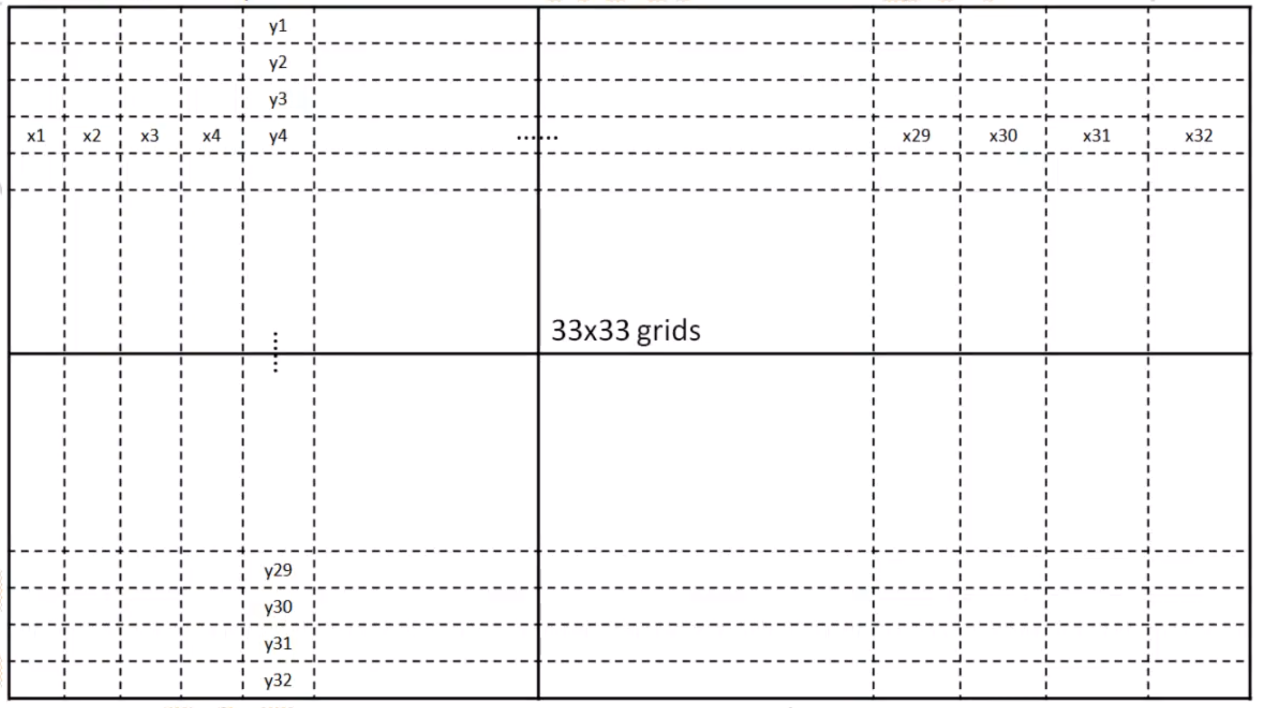
Figure 3.7‑1 LSC Region Division

Each region’s coordinates are programmable. Additionally, the lens shading correction parameters for each region and each color component are programmable. Each coordinate applies to each color component.

Within each sector, the correction function F(x,y) is expressed as a bilinear interpolation between discrete correction values at its four edges. This interpolation is performed in real-time by hardware during image processing.

Key Shading Parameters

LSC module parameters are located in VTunerClient under Lens Shading Correction.

Parameter	Type	Range	Description	Default Value
enable	bool	{true, false}	Enable the LSC module	false
matrix[4][33][33]	int[4][33][33]	[1024, 16383]	The gain of LSC, in R, Gr, Gb, B order.	All set to 1024
xSize[32]	int[32]	[0, width/2]	X stands for diffs The sum of 32 elements is equal to the width of the image	1080p: [60, 60, 60, 60, 60, 60, 60, 60, 60, 60, 60, 60, 60, 60, 60, 60, 60, 60, 60, 60, 60, 60, 60, 60, 60, 60, 60, 60, 60, 60, 60, 60]
ySize[16]	int[16]	[0, height/2]	Y stands for diffs The sum of 16 or 32 elements is equal to the height of the image Currently only 16 elements is supported.	[34, 34, 34, 33, 34, 34, 34, 33, 34, 34, 34, 33, 34, 34, 34, 33]

Table 3.7‑1 LSC Tuning Parameters

Static Calibration Key Parameters

LSC static calibration supports multiple color temperature correction tables. At least three color temperatures (high, medium, low) must be calibrated.

Parameter name	Description
Shading_ls_d65_[R/Gr/Gb/B]	Shading_ls_d65_[ R/Gr/Gb/B] D65 Shading table
Shading_ls_d50_[R/Gr/Gb/B]	Shading_ls_d65_[ R/Gr/Gb/B] D50 Shading table
Shading_ls_tl84_[ R/Gr/Gb/B]	Shading_ls_tl84_[ R/Gr/Gb/B] TL84 Shading table
Shading_ls_cwf_[R/Gr/Gb/B]	Shading_ls_d65_[ R/Gr/Gb/B] CWF Shading table
Shading_ls_a_[ R/Gr/Gb/B]	Shading_ls_a_[ R/Gr/Gb/B] A Shading table
Shading_ls_h_[R/Gr/Gb/B]	Shading_ls_d65_[ R/Gr/Gb/B] H Shading table

Table 3.7‑2 Mesh-based Lens Shading Static Calibration Parameters

Note: [R / Gr /Gb/ B] indicates separate labels/parameters for each color channel in the Bayer domain

The maximum gain value generated by Lens Shading is configurable, supporting up to 16x gain. The maximum compensation value for the lens can be configured during calibration using the calibration tool.

Tuning during phase one

Since Shading calibration depends on module characteristics, after meeting the prerequisites in Table 3.7-3, the tuning process can begin. Follow the corresponding section in the “X5-Calibration Tool User Guide” document to calibrate parameters.

Prerequisite	Status / value
Black level	Tuned
Gamma FE/BE	Tuned (Native WDR only)

Table 3.7‑3 Shading Calibration Prerequisites

Fine tuning lens shading phase three

Lens shading correction is a front-end module in the pipeline. By phase three, basic parameters have been adjusted, and only fine-tuning is needed based on real-world application requirements across various scenarios.

Tuning Process

In Auto mode, adjust the correction strength via the strength parameter, which is matched to gain gradients. For each gain gradient, find the correct shading strength setting for the current scene.

At low gain (high scene brightness), strength need not be reduced. As brightness decreases and gain increases, image noise increases. To maintain overall image quality—especially corner noise—shading strength can be reduced. In special cases, strength can be set to “0” (for lower corner brightness).

Additionally, the 2DNR module has noise reduction capabilities for shading and can be combined with shading strength. If 2DNR cannot eliminate all corner noise without causing blur, shading strength should be reduced to suppress noise.

Shading strength should be adjusted based on subjective assessment of visible noise. To obtain the correct strength value for each gain, adjust ambient brightness to achieve different gain levels.

Subjective Scene Tuning Method for Shading

1. Place the camera in a studio environment, preferably with gray flat areas at the corners. Ensure the current gain is 1x, which typically yields the best shading performance with minimal corner noise. Thus, shading strength can be set to maximum at this gain level. At high gain and low ambient brightness, assess corner noise and determine shading strength using the method described above.

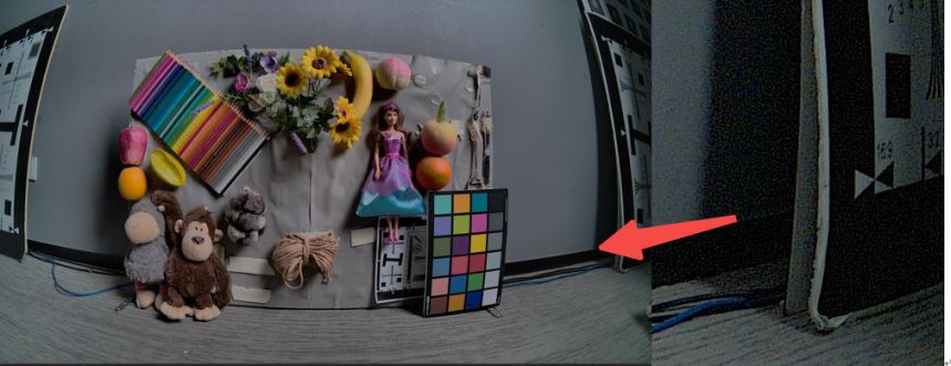
Figure 3.7‑2 ISP Gain 0, 1000 lux Scene

1. Reduce ambient brightness and increase gain to reach the next gain gradient. Subjectively evaluate noise level to determine the strength value for the current state. Set this value in the corresponding gain level of shading strength. Repeat this process for all gain levels to match appropriate shading strength values.

Figure 3.7‑3 ISP Gain 3, 500 lux Scene

For example, in a 500 lux scene, gain is approximately 3x. At this point, noise begins to increase, so slightly reducing shading strength for gain 3 is acceptable.

Figure 3.7‑4 ISP Max Gain, 20 lux – Max Strength

Figure 3.7‑5 Max Gain – Low Strength

Under 20 lux low-light conditions, maximum gain is often reached. Figure 3.7‑4 shows the image with maximum shading correction strength, while Figure 3.7‑5 shows the result after appropriately reducing shading strength. Reducing shading strength reduces image noise, though corner brightness decreases slightly. However, object information in the scene remains visible. During tuning, a trade-off between corner brightness and noise performance should be made based on actual requirements to achieve optimal image quality.

Digital Gain

Overview

Digital Gain is primarily used to increase image brightness. The input pixel value is multiplied by the gain value to produce the Digital Gain output. Each color component of the input RGB Bayer data is multiplied by the corresponding gain value in the DIGITAL_GAIN_x register. A gain value of 256 corresponds to a factor of 1.0, so the product of the color component and gain is right-shifted by 8 bits (rounded).

Tuning Theory

Calculation method for Digital Gain:

Figure 3.8‑1 Digital Gain Calculation Method

Digital Gain related parameters are as follows:

Parameter	Type	Range	Description	Default Value
enable	bool	{true,false}	Whether to enable Dgain module	true
digitalGainR	float	[1.0,255.0]	R gain	1.0
digitalGainGr	float	[1.0,255.0]	Gr gain	1.0
digitalGainGb	float	[1.0,255.0]	Gb gain	1.0
digitalGainB	float	[1.0,255.0]	B gain	1.0

Table 3.8‑1 Digital Gain Tuning Parameters

WDR

Overview

Wide Dynamic Range (WDR) technology is an advanced image processing method that significantly enhances both local and global contrast in images, making image details richer—especially in high-dynamic-range scenes such as backlit environments or shadow-heavy areas.

Tuning Theory

WDR is a method combining global and local tone mapping, used to compress bit depth to 12 bits and enhance image visibility. The core function of the module is to process the smallest unit of the image: a 16x16 pixel block. Depending on the input image resolution, the entire image is divided into multiple such blocks.

To achieve smooth visual transitions between blocks, the WDR module uses a bilateral filter for interpolation. This filter smooths subtle changes in color space while preserving edge clarity, creating seamless connections between blocks.

WDR enables control over processing intensity in different brightness regions. The module can independently adjust processing strength for low-brightness (low), high-brightness (high), and global (global) areas to achieve optimal image quality. In HDR digital overlap (DOL) mode, WDR relies on the exposure ratio between long and short frames to optimize the image.

Additionally, the WDR module offers two smoothing strength configuration modes:

Global Mode: All blocks use the same smoothing strength, ensuring consistent visual appearance across the entire image.

Local Mode: Smoothing strength can be adjusted based on brightness and content differences between blocks. This allows different processing intensities in different image regions, better handling local lighting variations.

Through these methods, the WDR module effectively adjusts local and global contrast, especially in backlit scenes or shadowed areas, providing clearer and more detailed image results.

General data processing flow:

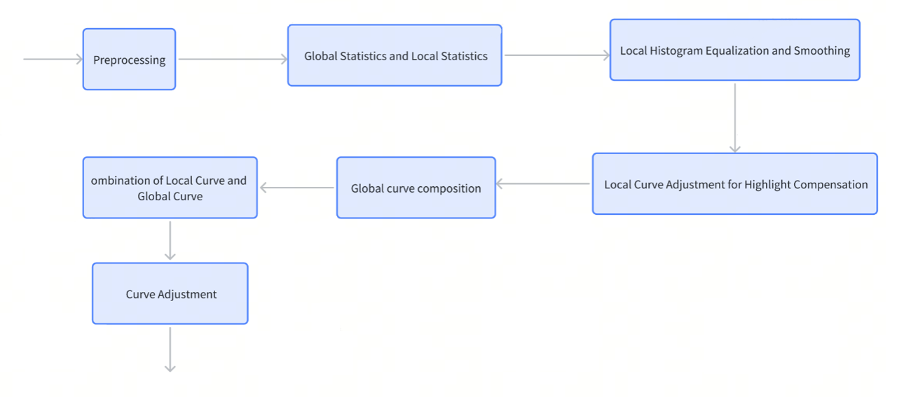
Figure 3.9‑1 WDR Processing Flowchart

Preprocessing

In image processing, especially in Wide Dynamic Range (WDR) applications, preprocessing of raw image data is a crucial step. The preprocessing flowchart is as follows.

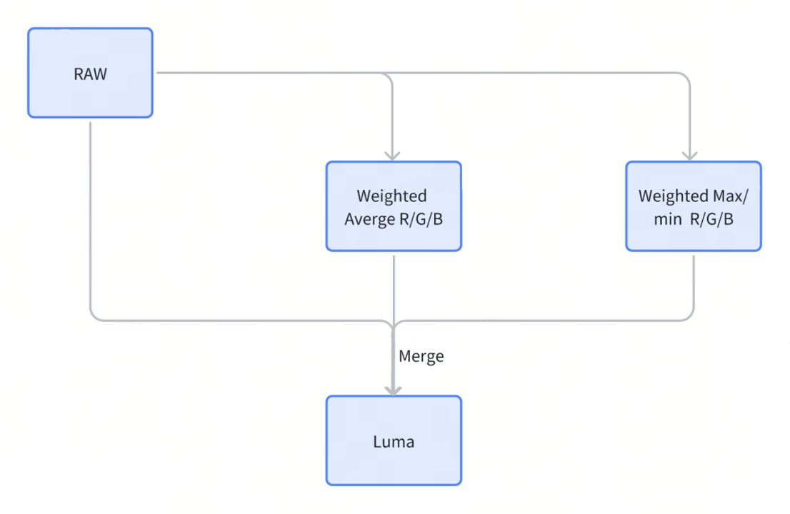
Figure 3.9‑2 WDR Preprocessing Diagram

The following are detailed descriptions of two key steps in preprocessing raw input images:

1. Luma Value Calculation. The first step in preprocessing is calculating the luma (brightness) value. This involves the following sub-steps:

 

1. Using a 3x3 pixel window, first calculate the weighted average of red (R), green (G), and blue (B) values.

2. Calculate the weighted sum of the maximum and minimum R/G/B values.

3. Combine the above two results with the input raw data to obtain the final luma value.

 

1. Pre-Gamma Mapping. Apply pre-gamma mapping and the low_strength module to further process the luma value. Pre-Gamma LUT is a lookup table with 65 bins used to expand grayscale values, making them more dispersed and enhancing the image’s dynamic range. Low_Strength is a configurable parameter used to control brightness in dark areas. A higher value results in richer brightness information in dark regions, increasing overall brightness.

After completing the above preprocessing steps, global and local statistics are performed on the luma values.

Global Statistics: Calculate the mean and standard deviation of the entire image to obtain overall brightness and contrast information.

Local Statistics: Divide the image into 16x16 pixel blocks and compute local curves for each block separately. This includes calculating the mean and histogram for each block, where the 20-bit grayscale values are divided into 64 bins and configured via a histogram LUT.

These preprocessing steps provide essential data for the WDR algorithm to optimize local and global contrast, especially in high-dynamic-range scenes such as backlit or shadowed areas.

Parameter	Type	Range	Description	Default Value
wdrLightnessWeight	int	[0,128]	max_rgb_weight	128
wdrColorWeight[3]	Int[3]	[0,128]	[gray_weight, lightness_weight, raw_weight] gray_weight + lightness_weight + raw_weight = 128	[128,0,0]

Table 3.9‑1 WDR Preprocessing Tuning Parameters

Local Histogram Equalization and Smoothing

Based on the histogram LUT, histogram statistics for each block can be obtained. Normalizing these statistics yields a local histogram curve. To prevent clipping or severe noise due to over-stretching, a 1D Gaussian smoothing is applied to the local curve. The smoothing index represents the smoothing level—the higher the index, the stronger the smoothing. Examples of image effects at different smoothing levels are shown below.

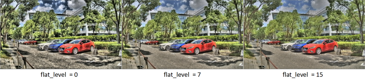
Figure 3.8‑3 Flat Level Smoothing Effect Example

There are two calculation modes for computing the smoothing level:

1. Manual Mode. All blocks directly use the flat_level value.

2. Semi-Automatic Mode. flat_level serves as the initial smoothing level, and each block’s flat index is calculated based on local histogram information and the configurable ISP_WDR5_LUT_FLAT_LEVEL_WRITE_DATA.

Local smoothing calculation related parameters are as follows.

Parameter	Type	Range	Description	Default Value
flatMode	bool	{true,false}	Strength adjustment mode for local contrast enhancement. false: Manual mode true: Auto mode (manual part + automatic incremental part)	false
flatLevel	int	[0,15]	Manual strength of local contrast enhancement The higher the value, the lower the manual strength.	5
flatLevelInc[4][17]	int[4][17]	[0,15]	Automatic incremental strength of local contrast enhancement The higher the value, the lower the automatic incremental strength.	[[3, 2, 1, 0, 0, 0, 0, 0, 0, 0, 0, 0, 0, 0, 0, 0, 0], [5, 4, 3, 2, 1, 0, 0, 0, 0, 0, 0, 0, 0, 0, 0, 0, 0], [7, 6, 5, 4, 3, 2, 1, 0, 0, 0, 0, 0, 0, 0, 0, 0, 0], [10, 10, 9, 8, 7, 6, 5, 4, 3, 2, 1, 0, 0, 0, 0, 0, 0]]
darkAttentionLevel	int	[0,14]	The level of attention to dark areas. The higher the value, the less attention to the dark area.	0

Table 3.9‑2 WDR LTM Tuning Parameters

Combination of Local Curve and Global Curve

In the merging process of local and global curves, the most important aspect is weight calculation. When contrast = 1023, the local curve weight is 1 and the global curve weight is 0—only the local curve takes effect. When contrast = 0, the local curve weight is 0 and the global curve weight is 1—only the global curve takes effect. When contrast is between (0,1023), the local and global curves are combined proportionally. Generally, using the local curve improves image contrast, while using the global curve reveals more detail in dark areas. During tuning, select an appropriate combination ratio based on actual needs.

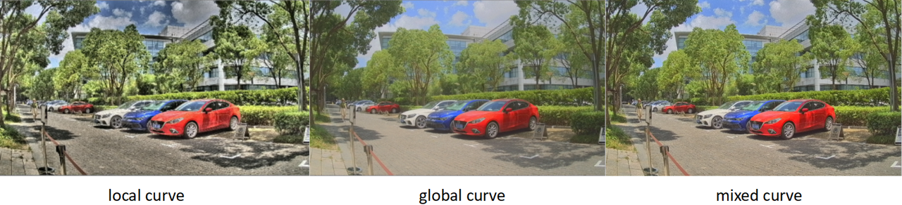
Figure 3.8‑4 Example of Local Curve and Global Curve Combination

If entropyEnable is enabled, the entropy and contrast of each block are used to calculate the merging strength of the global and local curves, which is then interpolated using gamma_down_lut. Finally, the local and global curves are merged using the computed strength.

Parameter	Type	Range	Description	Default Value
enable	bool	{true,false}	Enable/disable the WDR module	false
strength	int	[0,128]	As a fixed value of 128 when stitching is disabled, and as a variable value between 0~128 when stitching is enabled (0-base frame without WDR5, 128-stitching frame with WDR5).	128
highStrength	int	[0,128]	The larger the value, the richer the highlight information and the darker the global brightness.	0
lowStrength	int	[0,256]	The larger the value, the richer the lowlight information and the brighter the global brightness.	256
contrast	int	[-1023, 1023]	The larger the value, the stronger the local contrast.	0
entropyEnable	bool	{true,false}	true: Entropy information participates in block classification	false
entropySlope	int	[0,1023]	The larger the base, the smaller the slope, and the stronger the local contrast.	0
entropyBase	int	[0,1023]	The larger the base, the smaller the slope, and the stronger the local contrast.	0
wdrLumaThr	int	[0,1023]	Threshold of dark and bright area. entropyEnable=1: the parameter is invalid	64
fixedWeight	int	[0,1023]	Manual weight of global curve	0
flatLevelGlobal	int	[0,15]	Strength of auto global contrast enhancement The higher the value, the lower the strength.	5

Table 3.9‑3 WDR Strength Tuning Parameters

Curve Adjustment

In current ISPs, WB, CCM, and Gamma significantly affect color. Since CCM calibration is tied to Gamma, Gamma should remain enabled to ensure color accuracy. However, both WDR and Gamma increase image brightness, which can easily lead to overexposure if not properly adjusted. Therefore, a Degamma function is added within the WDR module to appropriately suppress brightness and prevent overly bright output.

WDR can reasonably distribute gray levels, simultaneously enhancing dark areas and suppressing bright areas, ensuring all pixels fall within the visible range. maxGain and minGain limit the gain applied to pixels of different brightness, preventing local overexposure and suppressing noise in dark areas. However, enhancing dark areas may amplify noise and color deviation, while suppressing bright areas may cause color artifacts near overexposed regions. Therefore, the final curve is constrained here. The WDR module allows for appropriate saturation reduction based on block gain values to suppress color deviation.

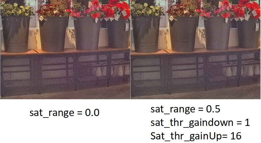
Figure 3.8‑5 WDR Dark Area Saturation Reduction Example

Additionally, WDR can moderately suppress high-contrast edges in the image. When edge contrast exceeds the set threshold diffHigh, the edge is softened to reduce contrast. Edges with contrast below diffLow are left unchanged. Edges with contrast between diffHigh and diffLow are interpolated and optimized.

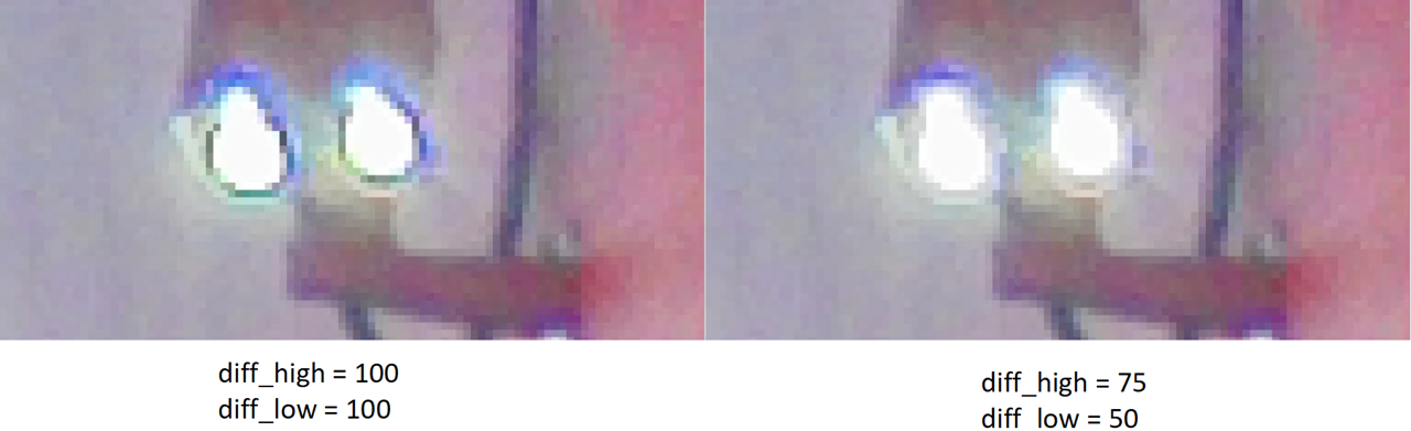
Figure 3.8‑6 WDR High-Contrast Edge Suppression

WDR curve adjustment parameters are listed in the table below:

Parameter	Type	Range	Description	Default Value
degamma	double	(0,3.0]	The factor of degamma curve The higher the value, the darker the image.	false
maxGain	int	[0,128]	Maximum of WDR gain	128

---

| minGain | int | [0,4096] | Minimum of WDR gain | 1 | | diffHigh | float | [0,100] | The threshold for detecting high contrast edges where the detected high contrast edges will become lighter in color. The higher the value, the fewer high-contrast edges are detected. | 100 | | diffLow | float | [0,100] | The threshold for detecting low contrast edges where the detected low contrast edges will become lighter in color. The higher the value, the fewer low-contrast edges are detected. | 100 | | satRange | float | [0,1] | Strength of saturation reduction | 0 | | satThrGainDown | int | [0,256] | The threshold used to determine pixels that need to be desaturated. The higher the value, the fewer dark pixels are desaturated. | 1 | | satThrGainUp | int | [0,256] | Refer to previous row. (This function can be used to reduce dark color noise and dark abnormal colors.) | 16 | | wdrRgbCoef | Int[3] | [0,128] | [weight_r, weight_g, weight_b] weight_r + weight_g + weight_b = 128 | [38,75,15] |

Table 3.9‑4 WDR Strength Tuning Parameters

Damping Function

Damping function is used to solve the flickering problem caused by scene changes in WDR. The root cause of flickering is the difference between the captured frame and the applied frame during scene changes — the curve generated from the captured frame is not applied to the current frame, and the curve changes gradually from frame to frame. WDR damping smooths the curve of data across frames in the time domain to mitigate flickering caused by scene changes.

Set dampMode to 0 (manual mode), then dampCurveCoef and dampAvgCoef must be set to values greater than 0 to ensure normal convergence and automatic adjustment of the WDR module. Set dampMode to 1 (auto mode), WDR will adaptively calculate dampCurveCoef and dampAvgCoef based on configured WDR parameters and the brightness distribution of the image.

WDR damping-related parameters are shown in Table 3.9-5.

Parameter	Type	Range	Description	Default Value
dampMode	int	{0,1}	0: Manual mode (damping coefficient can be configured directly) 1: Auto mode (damping coefficient is calculated adaptively according to the detection result of scene change)	0
dampCurveCoef	int	[0,127]	The damping parameter of the local curve. (manual mode valid) The larger the value, the faster the image brightness converges.	127
dampCurveMax	int	[0,127]	Limit of curve damping coefficient (auto mode)	127
dampCurveMin	int	[0,127]	Limit of curve damping coefficient (auto mode)	0
dampAvgCoef	int	[0,127]	Block mean luma damping coefficient (manual mode)	127
dampAvgMax	int	[0,127]	Limit of block mean luma damping coefficient (auto mode)	127
dampAvgMin	int	[0,127]	Limit of block mean luma damping coefficient (auto mode)	0
dampCoefDecLimit	int	[0,127]	Single step change limit of damping coefficient (auto mode)	127
dampCoefIncLimit	int	[0,127]	Single step change limit of damping coefficient (auto mode)	127
dampFilterSize	int	[0,16]	Reference frame number for scene change detection (auto mode)	8
dampLothrLog	float	[0.0,20.0]	Threshold for scene change detection (auto mode) The higher the value, the faster the video brightness converges.	0
dampHithrLog	float	[0.0,20.0]	Refer to the previous row	12

Table 3.9‑5 WDR Convergence Tuning Parameters

Halo Color Fading

This function operates in the HSV color space and primarily adjusts individual pixel saturation by tuning saturation thresholds and parameters for six pure colors (red, green, blue, yellow, cyan, magenta). These six pure colors divide the entire color space into six intervals. If a pixel falls within a certain interval, it will be adjusted only based on its two adjacent hue parameters. As shown in Figure 3.9‑7, only the R and Y parameters are effective at point a.

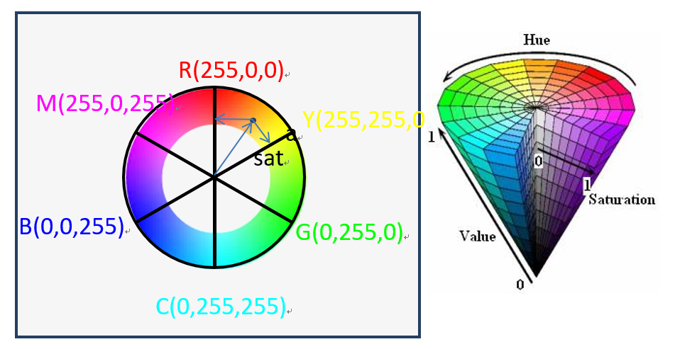
Figure 3.9‑7 WDR Preprocessing Diagram

Parameter	Type	Range	Description	Default Value
lightEnable	int	{0,1}	0: Halo color fading function disable 1: Halo color fading function enable	0
lightSatLothr	int	[0,255]	The low threshold of the saturation. pixel_sat ≤ lothr: the pixel is at low saturation, no need to desaturate. lothr < pixel_sat ≤ hithr: transition interval pixel_sat > hithr: the pixel is at high saturation, need to desaturate.	64
lightSatHithr	int	[0,255]	The high threshold of the saturation.	128
lightRedThrLog[4]	float[4]	[0.0,20.0]	Red threshold, monotonically increasing Logarithmic domain (same below)	[0,0,0,0]
lightGreenThrLog[4]	float[4]	[0.0,20.0]	Green threshold, monotonically increasing	[0,0,0,0]
lightBlueThrLog[4]	float[4]	[0.0,20.0]	Blue threshold, monotonically increasing	[0,0,0,0]
lightYellowThrLog[4]	float[4]	[0.0,20.0]	Yellow threshold, monotonically increasing	[0,0,0,0]
lightCyanThrLog[4]	float[4]	[0.0,20.0]	Cyan threshold, monotonically increasing	[0,0,0,0]
lightMagentaThrLog[4]	float[4]	[0.0,20.0]	Magenta threshold, monotonically increasing	[0,0,0,0]

Table 3.9‑6 WDR Halo Color Fading Tuning Parameters

When a pixel’s saturation reaches the adjustment threshold, its adjacent pure color parameters are also considered. Each hue is divided into five segments:

• pixel_value <= thr[0]: desaturation ratio is zero, used to protect low-saturation pixels.

• thr[0] < pixel_value <= thr[1]: the larger the pixel value, the greater the desaturation ratio, used for transition to eliminate purple fringing.

• thr[1] < pixel_value <= thr[2]: desaturation ratio is 1, used to reduce saturation.

• thr[2] < pixel_value <= thr[3]: the larger the pixel value, the smaller the desaturation ratio; used to increase halo color attenuation, creating a color absorption effect.

• pixel_value > thr[3]: desaturation ratio is zero, used to protect the color at the center of the light source.

To maintain color monotonicity, color_thr[0] and color_thr[1] are typically set to 0. However, if this function is used to reduce purple fringing, color_thr[2] and color_thr[3] should be set to the maximum value (20).

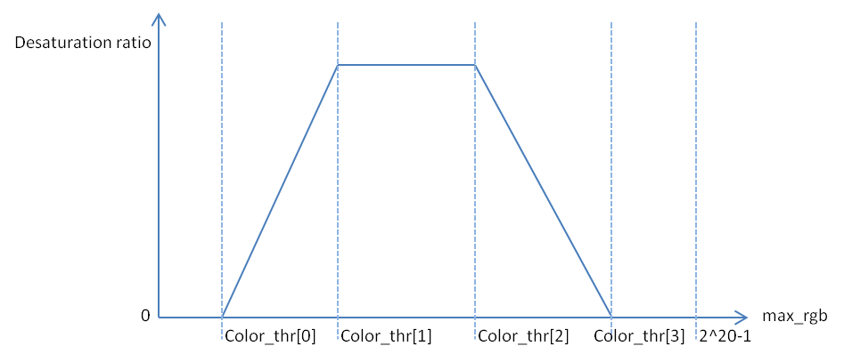
Figure 3.9‑8 WDR Highlight Color Suppression Schematic

Highlight Suppression

To handle scenes with light sources at night, a highlight suppression function has been added. The valid range of the local histogram is used to identify light sources. ISP_WDR5_HLC_CTRL is used to adjust the local histogram curve.

This function calculates the likelihood of a current block being a highlight region based on local contrast. The higher the likelihood, the greater the degree of light attenuation.

Parameter	Type	Range	Description	Default Value
hlcBaseLog	float	[0.0,19.0]	Highlight compensation threshold (logarithmic domain) The higher the value, the fewer highlight blocks are detected.	0.0
hlcSlope	int	[0,256]	Highlight compensation strength The higher the value, the stronger the highlight compensation.	0

Table 3.9‑7 WDR High Light Suppression Tuning Parameters

Green Equalization (GE)

Overview

The GE module is designed to balance the differences between adjacent gr and gb pixels in the original Bayer format and correct imbalances between the two pixels. Correcting imbalances can reduce checkerboard patterns or other similar artifacts generated by the demosaic interpolation algorithm, and can also improve false color performance in the demosaic algorithm. Figure 3.10‑1 illustrates how imbalances are identified:

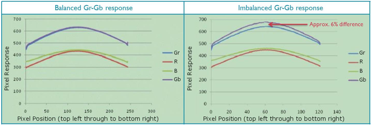
Figure 3.10‑1 GrGb Imbalance Schematic

Modern sensors rarely exhibit Green imbalance, meaning the default Green equalization values are generally acceptable. Older or lower-quality sensors may require tuning.

Regardless, the GE module requires validation, and the process is as follows:

• Phase one: No GE tuning required.

• Phase two: GE must be validated before demosaic tuning.

• Phase three: No GE tuning required.

Tuning Theory

Key Parameters of the GE Module

GE module parameters are included in the VTunerClient under Green Equalization. Specific descriptions are listed in the table below.

Parameter	Type	Range	Description	Default Value
enable	bool	{true, false}	Enable/disable GE module	true
threshold	float	[0,511]	The larger the threshold, the stronger the processing	2.5

Table 3.10‑1 GE Tuning Parameters.

Tuning GE during phase two

Since GE is not corrected in phase one, tuning occurs in phase two, before demosaic tuning. The prerequisites for tuning are as follows:

Prerequisite	Status / value
Black level	Tuned
Noise profile	Derived

Table 3.10‑2 GE Prerequisites

If Green imbalance is present, increase the GE_threshold parameter. This value can be set in the .json file. In phase three, re-tuning GE is generally not required unless GE introduces new issues.

Defect Pixel Cluster Correction (DPCC)

Overview

For various high- and low-end sensors, due to manufacturing processes, peripheral circuits, operating environments, and other factors, defective pixels inevitably appear during actual use. Defective pixels can be categorized as follows:

• Hot pixels: pixels that remain continuously bright

• Dead pixels: pixels that remain continuously dark

• Weak pixels: pixels that do not respond linearly to ambient light

Different types of defective pixels affect image quality differently. Dead pixels have minimal impact, while weak pixels are harder to predict. The DPC function mainly handles easily noticeable hot pixels. The complexity of handling hot pixels varies depending on their proximity, leading to the following classifications:

• Single hot pixel: an isolated hot pixel surrounded by normal pixels

• Double hot pixel: two adjacent hot pixels on the same color plane

• Triple hot pixel: three adjacent hot pixels on the same color plane

• Hot pixel cluster: four or more adjacent hot pixels on the same color plane

The DPCC tuning process is as follows:

• Phase one: no tuning required

• Phase two: verify static DPC status and perform multi-scene DPC tuning in a lab environment

• Phase three: no tuning required, unless DPC tuning or modules dependent on DPC degrade image quality

Tuning Theory

Defect Pixel Cluster Correction (DPCC) detects and corrects individual pixels and small clusters of defects (up to 3x3 pixels) on raw Bayer image data, i.e., impulse noise. The integrated defect pixel table allows independent correction of up to 2048 fixed-position defects, regardless of real-time detection. Practical analysis shows that residual effects increase with the number of defective pixels in the same flat area. This residual effect is due to averaging with neighboring pixels — the more defective pixels, the greater the impact. Therefore, if the image contains many hot pixel clusters, confirmation and improvement from the CMOS sensor manufacturer are recommended, as this can significantly affect image quality.

The DPCC module performs three tasks: static defect pixel table control, dynamic defect pixel detection, and defect pixel correction.

Static Defect Pixels

Set bptEnable to true, bptNum to the number of static defective pixels to correct, and configure bptPosX/bptPosY with the coordinates of the static defective pixels to mark them as bad points. If bptNum is less than the number of configured bptPosX/bptPosY coordinate pairs, only the number specified by bptNum will be corrected.

bptOutMode determines the correction method for static defective pixels. See the parameter description in the table for details.

Dynamic Defect Pixel Detection

The DPCC module evaluates whether the center pixel is defective from five perspectives: pixel value, pixel value ranking, pixel value difference, gradient ranking, and gradient extreme value within a 5×5 neighborhood. The selection of evaluation methods and the channel used for evaluation can be configured via methodsSet and setUse. See the parameter descriptions in the table for configuration logic.

Defect Pixel Correction

The correction method for defective pixels is controlled by the outMode parameter, primarily adjusting whether the center pixel is included in median calculations across channels. See the parameter description in the table for configuration logic.

DPCC module parameters are included in the VTunerClient under Defect Pixel Cluster Correction. Detailed parameter descriptions are listed in the table below.

Parameter	Type	Range	Description	Default Value
enable	bool	{true, false}	Enable/disable DPCC	false
bptEnable	bool	{true, false}	Enable static bad point correction	false
bptNum	int	[0,1024]	The number of static bad points	0
bptOutMode	int	[0,15]	Output mode for static bad-point correction. bptOutMode is a binary parsed parameter, with the following digits and corresponding functions: The first bit determines the G-channel. When using median filtering to calculate the correction value, whether the median filtering range includes the center point, 1 indicates yes and 0 indicates no. The second bit determines the RB channel. When using median filtering to calculate the correction value, whether the median filtering range includes the center point, 1 indicates yes and 0 indicates no. The third bit determines the G-channel. When using median filtering to calculate the correction value, whether the median filtering range uses all the same channel points within the 5x5 range, with 1 indicating yes and 0 indicating no. The fourth bit determines the RB channel. When using median filtering to calculate the correction value, whether the median filtering range uses all the same channel points within the 5x5 range, with 1 indicating yes and 0 indicating no.	0
bptPosX[2048]	int[2048]	[0, input_image_width]	The x-coordinate of the static bad point	[0]
bptPosY[2048]	int[2048]	[0, input_image_height]	The y-coordinate of the static bad point	[0]
outMode	int	[0,15]	Interpolation mode for correction unit outMode is a binary parsed parameter, with the following digits and corresponding functions: The first bit determines the G-channel. When using median filtering to calculate the correction value, whether the median filtering range includes the center point, 1 indicates yes and 0 indicates no. The second bit determines the RB channel. When using median filtering to calculate the correction value, whether the median filtering range includes the center point, 1 indicates yes and 0 indicates no. The third bit determines the G-channel. When using median filtering to calculate the correction value, whether the median filtering range uses all the same channel points within the 5x5 range, with 1 indicating yes and 0 indicating no. The fourth bit determines the RB channel. When using median filtering to calculate the correction value, whether the median filtering range uses all the same channel points within the 5x5 range, with 1 indicating yes and 0 indicating no.	0
setUse	int	[0,15]	DPCC methods set usage for detection The first bit determines whether the entire set of parameters for stg1 is enabled. The second digit determines whether the entire set of parameters for stg2 is enabled. The third digit determines whether the entire set of parameters for stg3 is enabled. Its fourth position is determining stg_ Whether the entire set of parameters for fix is enabled, that is, whether a built-in judgment mechanism is enabled.	1
methodsSet[3]	int[3]	[0,8191]	Methods enable bits for SET_1/2/3, different methods can be used in parallel, the result is the logical AND of all selected methods. methodsSet is a 13-bit numerical value that needs to be viewed in binary. For all bits, 1: enabled; 0: disabled. Its lower 5 bits determine the activation of the five bad point detection methods for the G channel. The lowest bit determines whether the PG (peak gradient) method of the G channel is enabled. The second digit determines whether the LC method of channel G is enabled. The third digit determines whether the RO method of channel G is enabled. The fourth digit determines whether the RND method of channel G is enabled. The fifth digit determines whether the RG method of the G channel is enabled. The 9th to 13th positions determine the five methods for opening the RB channel. The 9th digit determines whether the PG (peak gradient) method of the RB channel is enabled The 10th digit determines whether the LC method of the RB channel is enabled. The 11th bit determines whether the RO method of the RB channel is enabled. The 12th digit determines whether the RND method of the RB channel is enabled. The 13th digit determines whether the RG method of the RB channel is enabled.	[1, 7453, 0]
lineThresh[2][3]	int[2][3]	[0, 255]	Line threshold methods, 3 thresh for RB and G	[[0, 0, 0], [0, 0, 0]]
lineMadFac[2][3]	int[2][3]	[0,63]	Mean Absolute Difference (MAD) factor for Line check	[[0, 0, 0], [0, 0, 0]]
pgFac[2][3]	int[2][3]	[0,63]	Peak gradient factor	[[0, 0, 0], [0, 0, 0]]
rndThresh[2][3]	int[2][3]	[0, 255]	Rank Neighbor Difference threshold	[[0, 0, 0], [0, 0, 0]]
rgFac[2][3]	int[2][3]	[0,63]	Rank gradient factor	[[0, 0, 0], [0, 0, 0]]
roLimits[2][3]	int[2][3]	[0,3]	Rank Order Limits	[[0, 0, 0], [0, 0, 0]]
rndOffs[2][3]	int[2][3]	[0,3]	Differential Rank Offsets for Rank Neighbor Difference	[[0, 0, 0], [0, 0, 0]]

Table 3.11‑1 DPCC Tuning Parameters

Tuning DPC during phase two

DPCC module tuning is not required in phase one; related tuning is performed in phase two. Before tuning, parameters must be preset and related modules tuned. Presetting can be done in two ways:

Method 1: Refer to the default configuration in Table 3.11‑1.

Method 2: Select one of the six preset parameter sets and tune based on it to generate a new configuration.

Tuning Procedure

1. Point the camera at the scene set up in the lab, as shown below. In VTunerClient, set exposure to Manual mode.

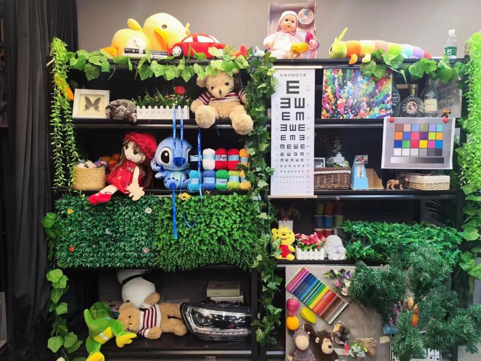
Figure 3.11‑1 Example of a studio scene

1. Enable DPCC by setting enable to 1, configure with default parameters from the table, and observe the distribution of defective hot pixels in the image.

2. If defective pixels are still visible under current parameters, decrease lineMadFac/lineThresh/rndThresh/rgFac, or increase roLimits/pgFac. Adjust in steps of about 10% of the parameter range until defective pixels are no longer visible.

3. Reduce the adjustment step size and fine-tune each parameter until defective pixels are successfully removed. These values represent the threshold for defect removal. Fine-tune as needed until the DPCC configuration meets specifications at the current gain, then save the configuration.

4. Repeat steps 3–4 to adjust DPCC parameters for all gain levels.

Fine tuning DPC during phase three

After completing fine tuning of the DPC module and adjusting DPCC parameters across different gain levels, write the corresponding parameter table into the configuration. If defective pixels are still observed in real-world scenarios, fine-tune the parameters for the corresponding gain level based on the specific scene.

2DNR

Overview

2D Noise Reduction (2DNR) module is used to reduce spatial noise in RAW images. It is a key component of the ISP, significantly improving image quality, especially for images captured under low-light conditions. The 2DNR module performs filtering at three layers — high, medium, and low — and outputs the final result.

2DNR can be divided into four main functions: filtering processing, detail enhancement, Luma control, and motion blending.

The general tuning process is as follows:

• Phase one: no adjustment required.

• Phase two: adjust 2DNR parameters in a real lab environment.

• Phase three: fine-tune 2DNR parameters for different real-world scenarios to achieve optimal performance across all conditions. This phase mainly adjusts 2DNR configuration parameters under different gain values.

Tuning Theory

NLM Processing

This module uses the Non-Local Means (NLM) algorithm to search within a large search window for pixel groups with features similar to the current pixel. By computing the weighted average of these points and using a Gaussian-like weighting function to accumulate all similar pixel blocks, it effectively eliminates random noise in the original pixel blocks, thereby significantly improving the Signal-to-Noise Ratio (SNR) of the image.

During 2DNR processing, to maximize algorithm performance, the camera’s noise profile must be used. During objective calibration, the noise profile must be accurately calibrated under different gain conditions. This is crucial to ensure the algorithm can properly adjust its processing strategy according to actual noise levels to optimize image quality. Additional NR TOOL usage instructions are provided.

2DNR processing flowchart:

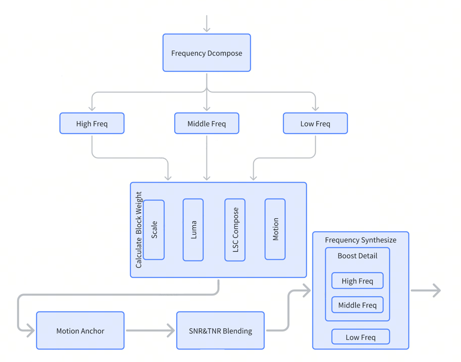
Figure 3.12‑1 2DNR Processing Flowchart

2DNR module parameters are included in the VTunerClient under 2D Noise Reduction.

Note: In this table, layer 0 refers to the detail layer, layer 1 to the medium-detail layer, and layer 2 to the coarse information layer.

Parameter	Type	Range	Description	Default Value
enable	int	[0,1]	0: disables 2DNR . 1: enables 2DNR .	0
vstFactor	float	[1.0, 1000.0]	A factor to control the sigma of the decompose filter. The greater the factor, the larger the decompose sigma.	16
motionCtrlEn	int	[0,1]	0: bypasses motion adaptive 2DNR. 1: enables motion adaptive 2DNR.	1
sigmaFactorMotionMin	int	[0, 1024]	The minimum 2DNR threshold. For pixels with motion less than this threshold, 0% 2DNR is applied.	0
sigmaFactorMotionMax	int	[1, 1024]	The maximum 2DNR threshold. For pixels with motion greater than this threshold, 100% 2DNR is applied.	800
sigmaScale[3]	float[3]	[0.001, 100.0]	The sigma factors for layer 0, layer 1, and layer 2 in order. A greater sigma factor makes the corresponding layer smoother.	[1.0, 1.0, 1.0]

Table 3.12‑1 2DNR NLM Tuning Parameters

Luma Control

lumaCurve is a key function in 2DNR processing that performs noise reduction based on pixel luminance. During this process, lumaCurveX and lumaCurveY are used together to adjust denoising strength according to pixel brightness. Specifically, the higher the value of lumaCurveY, the weaker the denoising effect. This allows effective noise reduction while preserving image details.

lscCompCurve adjusts noise reduction based on the distance between a pixel’s current position and the image center. The curve is designed so that denoising strength in edge regions can be adjusted based on distance from the center. The higher the value of lscCompCurve, the weaker the denoising effect, where 1024 corresponds to a multiplier of 1.0. This means that when lscCompCurve is 1024, the denoising effect is neither enhanced nor reduced.

Proper setting of these two curve parameters is critical for achieving high-quality image denoising. Users should adjust these parameters based on specific image content and desired denoising results.

Parameter	Type	Range	Description	Default Value
lumaCtrlEn	int	[0, 1]	0: bypasses luma adaptive 2DNR. 1: enables luma adaptive 2DNR.	1
lscGainCompEn	float	[0, 1]	0: disables gain compensation for lens shading compensation (LSC). 1: enables gain compensation for LSC.	0
lumaCurveX[12]	int[12]	[0,4095]	The luma control curve in SNR. Based on this curve, the local SNR sigma is adjusted according to the luma value of each pixel. The greater the value of lumaCurveY, the weaker the SNR denoising effect. Value 256 leads to the same SNR denoising effect as when lumaCtrlEn is set to 0 to disable luma control. lumaCurvePx indicates the base 2 logarithm of the distance between adjacent X anchors specified by is lumaCurveX. lumaCurvePx is reserved for compatibility and is usually not used.	[0, 32, 64, 96, 128, 256, 512, 768, 1024, 1536, 2048, 4095]
lumaCurveY[12]	int[12]	[0,65535]	[256, 256, 256, 256, 256, 256, 256, 256, 256, 256, 256, 256]
lumaCurvePx[12] consider removing	int[12]	[0,12]	[0, 5, 5, 5, 5, 7, 8, 8, 8, 9, 9, 11]
lscCompCurveX[12]	int[12]	[0,4095]	The LSC gain compensation curve in SNR. Based on this curve, the local SNR sigma is adjusted according to pixel coordinates. The greater the value of lscCompCurveY, the weaker the SNR denoising effect. Value 1024 leads to the same SNR denoising effect as when lscGainCompEn is set to 0 to disable gain compensation for LSC. lscCompCurvePx indicates the base 2 logarithm of the distance between adjacent X anchors specified by is lscCompCurveX. lscCompCurvePx is reserved for compatibility and is usually not used.	[0, 32, 64, 96, 128, 256, 512, 768, 1024, 1536, 2048, 4095]
lscCompCurveY[12]	int[12]	[0,65535]	[1024, 1024, 1024, 1024, 1024, 1024, 1024, 1024, 1024, 1024, 1024, 1024]
lscCompCurvePx[12] consider removing	int[12]	[0,12]	[0, 5, 5, 5, 5, 7, 8, 8, 8, 9, 9, 11]

Table 3.12‑2 2DNR Luma Control Tuning Parameters

Moving&Static Boosting

The 2DNR module can control detail enhancement in motion and static regions.

Parameter	Type	Range	Description	Default Value
motionFactorCurveX[12]	int[12]	[0, 1024]	The motion control curve in SNR. Based on this curve, the local SNR sigma is adjusted according to the motion value of each pixel. The greater the value of motionFactorCurveY, the weaker the SNR denoising effect. Value 128 leads to the same SNR denoising effect as when motionCtrlEn is set to 0 to disable motion control. motionFactorCurvePx indicates the base 2 logarithm of the distance between adjacent X anchors specified by is motionFactorCurveX. motionFactorCurvePx is reserved for compatibility and is usually not used.	[0, 4, 8, 16, 32, 64, 128, 192, 256, 384, 512, 1024]
motionFactorCurveY[12]	int[12]	[0, 65535]	[1408, 1152, 1024, 896, 768, 640, 512, 437, 384, 309, 256, 128]
motionFactorCurvePx[12]	int[12]	[0, 10]	[0, 2, 2, 3, 4, 5, 6, 6, 6, 7, 7, 9]
motionAnchorX[2]	int[2]	[0, 1024]	The motion thresholds. Pixels with motion less than motionAnchorX[0] are considered static and use static boost parameters. Pixels with motion greater than motionAnchorX[1] are considered moving and use moving boost parameters. For pixels with motion between motionAnchorX[0] and motionAnchorX[1], their boost threshold and clip threshold are obtained through linear interpolation	[100, 600]
staticDetailThresh[2][3]	int[2][3]	[0, 4095]	The detail suppression threshold for static pixels per layer per RGB channel. For instance, staticDetailThresh[0][1] indicates the threshold for static pixels at layer 0 for color channel 1. Coefficients of detail pixels that are less than the threshold are set to 0.	[[0, 0, 0], [0, 0, 0]]
staticDetailBoostThresh[2][3]	int[2][3]	[0, 4095]	The detail boosting threshold for static pixels per layer per RGB channel. For instance, staticDetailBoostThresh[0][1] indicates the threshold for static pixels at layer 0 for color channel 1.	[[4095, 4095, 4095], [4095, 4095, 4095]]
staticDetailBoost[2][3]	float[2][3]	[1.0, 4.0]	The detail boosting factor for static pixels per layer per RGB channel. For instance, if the detail amount of static pixels at layer 0 for color channel 1 is greater than staticDetailBoostThresh[0][1], the detail amount is multiplied by staticDetailBoost[0][1].	[[1.0, 1.0, 1.0], [1.0, 1.0, 1.0]]
staticDetailClipThresh[2][3]	int[2][3]	[0, 4095]	The detail boosting clipping threshold for static pixels per layer per RGB channel. For instance, staticDetailClipThresh[0][1] indicates the threshold for static pixels at layer 0 for color channel 1. The boosting value is calculated as follows: boosting value = clip(boost_fac × (detail_input − boost_thresh), clip_thresh)	[[4095, 4095, 4095], [4095, 4095, 4095]]
movingDetailThresh[2][3]	int[2][3]	[0, 4095]	The detail suppression threshold for moving pixels per layer per RGB channel. For instance, movingDetailThresh[0][1] indicates the threshold for moving pixels at layer 0 for color channel 1. Coefficients less than the threshold are set to 0.	[[0, 0, 0], [0, 0, 0]]
movingDetailBoostThresh[2][3]	int[2][3]	[0, 4095]	The detail boosting threshold for moving pixels per layer per RGB channel. For instance, movingDetailBoostThresh[0][1] indicates the threshold for moving pixels at layer 0 for color channel 1.	[[4095, 4095, 4095], [4095, 4095, 4095]]
movingDetailBoost[2][3]	float[2][3]	[1.0, 4.0]	The detail boosting factor for moving pixels per layer per RGB channel. For instance, if the detail amount of moving pixels at layer 0 for color channel 1 is greater than movingDetailBoostThresh[0][1], the detail amount is multiplied by movingDetailBoost[0][1].	[[1.0, 1.0, 1.0], [1.0, 1.0, 1.0]]
movingDetailClipThresh[2][3]	int[2][3]	[0, 4095]	The detail boosting clipping threshold for static pixels per layer per RGB channel. For instance, staticDetailClipThresh[0][1] indicates the threshold for static pixels at layer 0 for color channel 1. The boosting value is calculated as follows: boosting value = clip(boost_fac × (in − boost_thresh), clip_thresh)	[[4095, 4095, 4095], [4095, 4095, 4095]]
staticFactor[3]	float[3]	[0.01, 1.0]	The sigma ratio of fully static regions for each layer. If this parameter is set to 0.1, it means 0.1 × moving_sigma is applied to fully static pixels. It helps keep fine details in the background.	[0.1, 0.1, 0.1]
sigmaFactorMul[3]	float[3]	[0.1, 10.0]	The factor that adjusts the decreasing speed of SNR sigma from moving to static for each layer. A greater value of this parameter leads to stronger denoising effects in previously moving regions.	[1.0, 1.0, 1.0]

Table 3.12‑3 2DNR Motion&Static Boost Tuning Parameters

motionAnchorX Parameter Description:

The motionAnchorX parameter is used to distinguish whether a pixel is in a static or moving state during image enhancement (boosting). This parameter includes two key thresholds: motionAnchorX[0] and motionAnchorX[1].

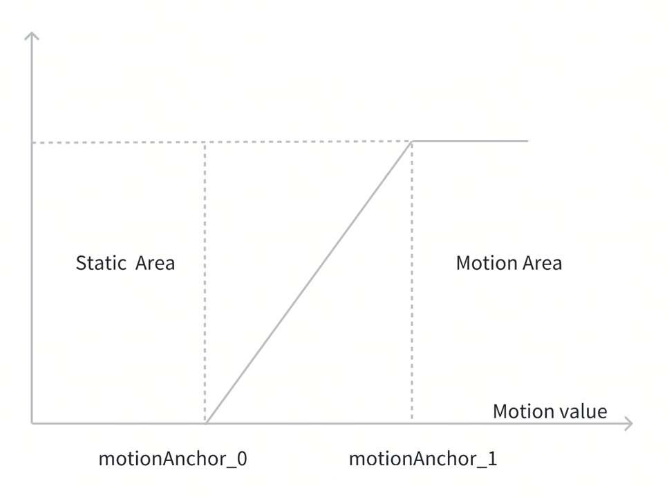
Figure 3.12‑2 2DNR MotionAnchor Function Schematic

When a pixel’s motion value is less than motionAnchorX[0], it is considered static. During boosting, the following static-state boosting parameters are used:

• Static detail threshold (static detail thresh)

• Static detail boost threshold (static detail boost thresh)

• Static detail boost (static detail boost)

• Static detail clip threshold (static detail clip thresh)

When a pixel’s motion value is greater than motionAnchorX[1], it is considered moving. During boosting, the following motion-state boosting parameters are used:

• Moving detail threshold (moving detail thresh)

• Moving detail boost threshold (moving detail boost thresh)

• Moving detail boost (moving detail boost)

• Moving detail clip threshold (moving detail clip thresh)

For pixels with motion values between motionAnchorX[0] and motionAnchorX[1], their threshold, boost threshold, boost, and clip threshold parameters are calculated via interpolation based on the static and motion parameter sets.

Frequency synthesis (Frequency Synthesis) is performed based on the pixel’s boosting parameters, as follows:

• If abs(detail) < threshold, output (out) = coarse layer.

• If abs(detail) > threshold and abs(detail) < boosting threshold, output (out) = coarse layer + detail layer.

• If abs(detail) > boosting threshold, output (out) = coarse layer + detail layer × boost factor, but not exceeding max boosting value.

Adjust the parameter values above according to your specific algorithm and application requirements.

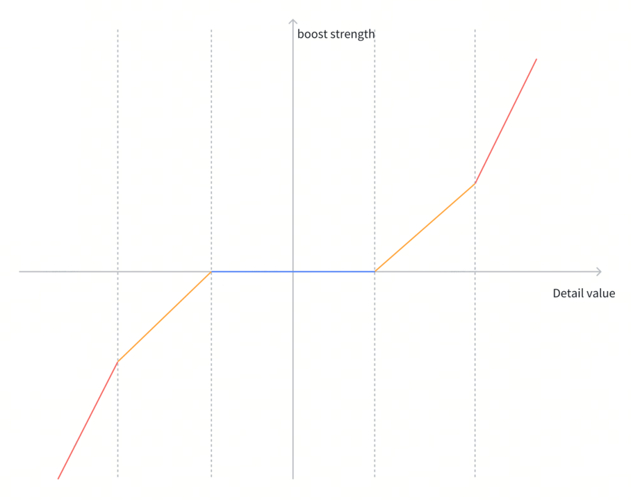
Figure 3.12‑3 2DNR Static&Motion Detail Boost Schematic

2DNR and 3DNR Blending

While the 2DNR algorithm effectively removes noise, it may also lead to loss of image detail. To balance noise reduction and detail preservation, the algorithm applies different weights to 2DNR based on whether a region is static or moving. Each pixel’s weight is determined by its local motion factor and adjusted via a motion control curve.

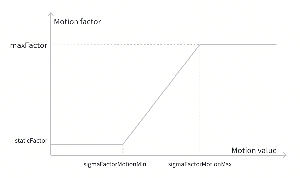
Figure 3.12‑4 Relationship between 2DNR and MotionFactor

Local SNR standard deviation adjustment: Adjust the local SNR standard deviation based on pixel motion via the motion control curve. A higher motionFactorCurveY value indicates weaker SNR denoising. When set to 128, it corresponds to a multiplier of 1.0 — no enhancement or reduction in denoising.

Processing of static region pixels:

Processing of fully moving region pixels:

Processing of pixels between static and moving regions:

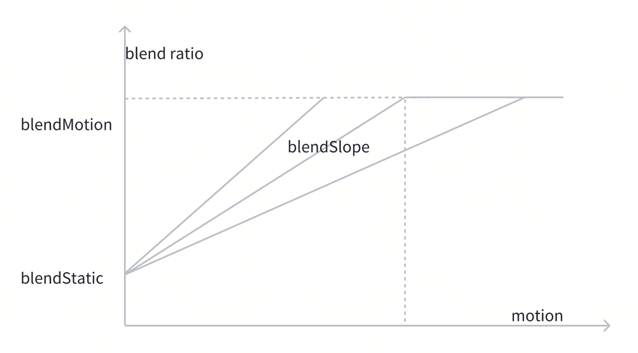
Figure 3.12‑5 Static&Motion 2DNR Blending Schematic

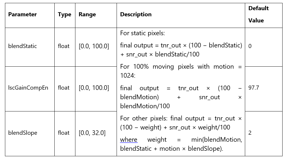
Table 3.12‑4 2DNR&3DNR Blending Tuning Parameters

Tuning 2DNR during phase two

Since 2DNR tuning does not depend on sensor characteristics, tuning begins in phase two. After meeting the prerequisites listed in the table below, proceed to the tuning process.

Module	Status / Value
Black level	Tuned
DPC	Tuned
Green equalization	Tuned
Demosaic	Tuned
3DNR	Tuned
noise profile	set

Table 3.12‑5 2DNR Prerequisites

The real-world scene used for 2DNR tuning should include a ColorChart, various textured props, multi-colored textures, flat areas, and an ISP12233 chart, to effectively observe the 2DNR module’s impact on various objects and regions.

Tuning Procedure

The general 2DNR tuning flowchart is shown in Figure 3.12‑6. To tune 2DNR to meet requirements, process and analyze a large number of images with different content, detail levels, and brightness, making both objective and subjective evaluations. Generally, under low gain, use smaller 2DNR threshold values to preserve texture and detail; under high gain, increase the 2DNR threshold to achieve better noise reduction.

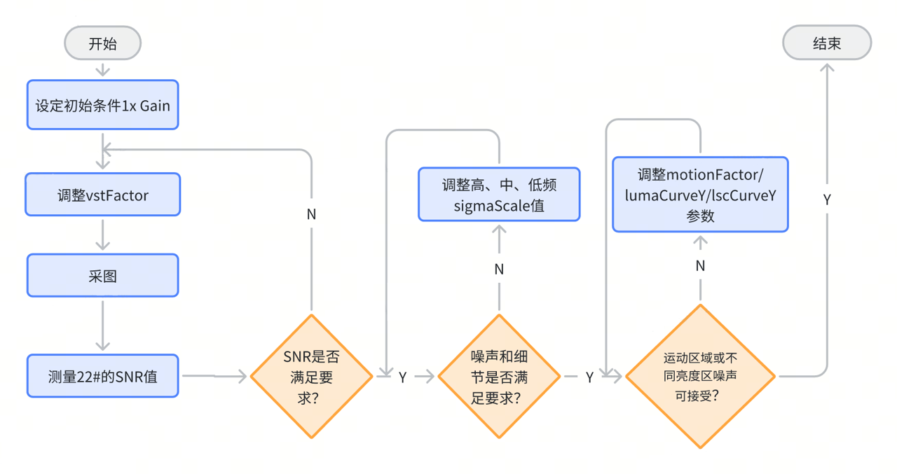
Figure 3.12‑6 2DNR Tuning Flowchart

2DNR Filtering Process

1. Similar Block Search

Use Sum of Absolute Differences (SAD) to compare the similarity between the search block and the center block.

1. Block Weight Calculation and Conversion

Use a Gaussian-like decreasing curve to convert SAD into block weights.

Sigma Calculation:

The larger the sigma value, the smoother the curve, the stronger the filtering effect, approaching mean filtering. vstFactor determines sigma, and sigmaScale determines the sigma scaling factor for each layer.

1. Sigma Factor Calculation

This factor adjusts SAD considering luminance, motion, and LSC compensation.

Luminance:

Motion:

• If motion < sigmaFactorMotionMin, motion_factor = staticFactor.

• If motion > sigmaFactorMotionMax, motion_factor = 64.

• Otherwise, motion_factor = LUT lookup(snr_motion_curve, motion_frame[i,j]) × sigma_factor_mul

1. Isc Gain

1. Block Weight Confirmation

Position of block in weight curve

sigma_offset sets a threshold relative to SAD; blocks with SAD below it receive maximum weight. The larger the above factors, the larger the final SAD, the weaker the filtering.

1. Calculate Final Block Weight

Compute weighted average of all blocks to determine final block weight.

Note: SNR is a noise evaluation metric but cannot reflect perceived noise and detail by the human eye, so it should not be used for subjective analysis.

Due to the high subjectivity of 2DNR tuning, it can be broken down into sub-modules, each tuned separately. The basic tuning flow is:

1. Set 2DNR default parameters according to Table 3.12‑6

Parameter	Default
Driver_load	False
Sigma	5
Pregamma_strength	1
Luma_curve_x	[0, 32, 64, 96, 128, 196, 256, 512, 768, 1024, 2048, 4096 ]
Luma_curve_y	[256, 256, 256, 256, 256, 240, 210, 180, 150, 200, 256, 256 ]

Table 3.12‑6 2DNR Default Parameters

1. Set Enable to 0 to disable the 2DNR module and capture a real-world image containing a ColorChecker at Total Gain 1x.

2. Use Imatest to analyze the SNR value of Patch22 (the fourth point in the figure below). This value will serve as the reference SNR after enabling 2DNR. Adjust 2DNR parameters based on SNR as follows:

Figure 3.12‑7 Imatest ColorChecker SNR Output

1. Set Enable to 1, observe and verify image quality. Carefully examine changes in texture details and SNR before and after.

2. If the required SNR is not met, readjust vstFactor until the desired SNR requirement is satisfied.

3. After the SNR basically meets the requirements, further evaluate whether the noise and detail performance in the image meet the requirements. If not, adjust the sigmaScale values corresponding to the high, medium, and low frequency domains.

4. Observe whether the noise levels in different brightness regions, from center to corner regions, and in motion areas meet the requirements. If not, adjust the values of lumaCurve, motionFacCurve, and lscCurveY until the requirements are met.

5. Adjust the environmental brightness to different Gain multiples, and repeat steps 2)–4) to fine-tune the 2DNR parameters.

Motion Blending

Dynamically adjust the strength of 2DNR based on the intensity of motion. The stronger the motion, the greater the 2DNR strength and the weaker the 3DNR strength, thereby improving SNR while reducing motion artifacts in moving regions.

Verification

After completing the adjustment of all parameters described above, capture images under different Gain conditions in a real-scene laboratory environment, and analyze the images using the ColorChecker module in Imatest. If both the SNR values and the texture detail performance meet the requirements, 2DNR can proceed to the third phase of tuning. Otherwise, repeat the above steps until the requirements are satisfied.

Additional Tuning Information

The data in Table 3.12-7 can be used as reference SNR values. Figure 3.12‑8 shows the actual effect when SNR > 40. From the image, it can be seen that both noise and texture are well preserved.

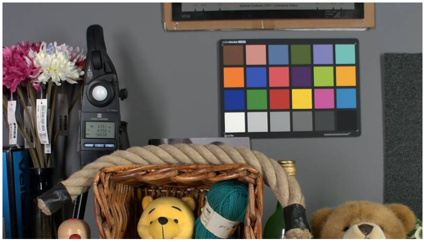
Figure 3.12‑8 Real-scene illustration of 2DNR tuning

D65 1x gain condition reference	Halogen lamp, system maximum Gain
Good: 40 - 50	Good: 25-35
Fair: 35 - 40	Fair: 15 - 25
Poor: < 35	Poor: < 15

Table 3.12‑7 Target SNR values

During tuning, balance noise and texture detail performance according to specific requirements. However, in most cases, avoid extreme parameter settings that result in excessive noise in the image.

Fine tuning 2DNR phase three

After completing parameter adjustments under different Total Gain conditions in the second phase, proceed to the third phase of tuning. Other modules in the ISP Pipeline may also affect 2DNR tuning. Therefore, to achieve a more balanced image quality across all gain conditions, jointly adjust the DPC, 2DNR, 3DNR, Demosaic, and EE modules according to the configured gain LUT.

Modern sensors exhibit almost no visible noise under good lighting conditions or at 1x Gain. In such cases, reduce the illumination until the Gain increases sufficiently to make noise visible in the image. For gain conditions with no visible noise, maintain relatively low noise reduction strength settings.

3DNR

Overview

3DNR combines spatial denoising based on edge/motion detection (non-local mean filter) and temporal denoising. The non-local filter primarily suppresses noise in static regions, while temporal filtering targets noise on moving objects. The motion detection module in 3DNR distinguishes between moving and non-moving regions. Temporal filtering and spatial denoising are applied separately to motion and static regions. Intermediate transition areas use a blend of spatial and temporal filtering for smoother output, ultimately generating a denoised frame.

For static regions, more reference values are used as tnr_out; otherwise, the current value is used. When computing motion regions, both motion_frame and motion_history (motion reference read from memory) are considered.

The 3DNR section includes the following sub-functions: Motion detection, Motion dilation, Motion Mask Blending, Reference Frame Blending, and NoiseProfile calibration.

Below is a brief description of the tuning process:

Phase One: Calibrate the module’s NoiseProfile.

Phase Two: Adjust 3DNR strength and motion parameters in a real-scene laboratory environment.

Phase Three: Fine-tune 3DNR parameters for real-world scenarios to ensure optimal performance across all conditions. This phase mainly involves adjusting 3DNR parameters under different Gain values.

Tuning Theory

The processing flowchart of the entire 3DNR module is shown below:

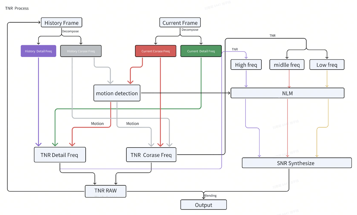
Figure 3.13‑1 3DNR Processing Flowchart

3DNR module parameters are included in the “2D Noise Reduction” section of VTunerClient. Detailed descriptions of tuning parameters are provided in the table below.

Parameter	Type	Range	Description	Default Value
enable	int	[0,1]	0: bypasses 3DNR v4. 1: enables 3DNR v4.	0
tnrEn	int	[0,1]	0: bypasses temporal noise reduction (TNR). 1: enables TNR.	1
nlmEn	int	[0,1]	0: bypasses spatial noise reduction (SNR). 1: enables SNR	1
motionDilateEn	int	[0,1]	0: disables motion dilation. 1: enables motion dilation.	0
gaussBlurEn	int	[0,1]	0: disables Gaussian blur before motion detection. 1: enables Gaussian blur before motion detection.	0
noiseModelEn	int	[0,1]	0: disables the noise model curve. 1: enables the noise model curve.	1
inputBits	int	{20,24}	The bit depth of the noise model curve.	20
noisemodelA	double	[0.1, 100]	The slope of the noise model curve. This parameter is calibration data used to calculate the noise curve by the driver.	0.3
noisemodelB	double	[0.1, 10000]	The offset of the noise model curve. This parameter is calibration data used to calculate the noise curve by the driver.	1.5

Table 3.13‑1 Basic Configuration Parameters of 3DNR

Calculation Process of Temporal Filtering

1. Calculation of historical reference frame length

Calculate the factor update during reference iteration:

The larger the filterLen, the larger the thr_update. This determines the length of the history window; a longer time window improves temporal noise reduction.

1. TNR Result Calculation

   

In NR4, detail and coarse layers undergo separate temporal filtering, and are blended back with tnr_in based on tnr strength and tnr_strength2 settings.

1. Update historical motion information

The larger the filterLen2, the larger the motion_thr_update. This affects the transition area of motion, mainly because different motion intensities affect 2DNR strength differently.

Motion Detection

The motion detection module is designed based on the original low- and mid-frequency data from reference and current frames, using two types of difference values—SAD and block mean—to estimate motion detection results. Block difference calculation is performed in the RGB domain.

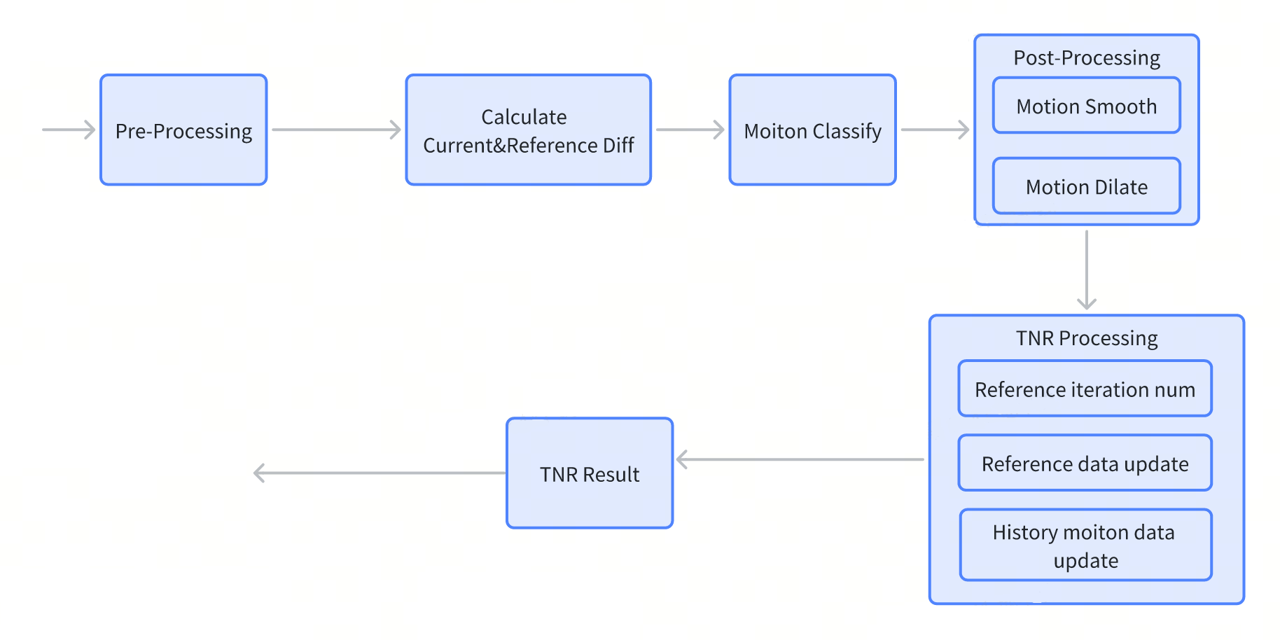
Figure 3.13‑2 3DNR Motion Detection Processing Flowchart

Motion Detection Processing Steps:

1. Pre-processing

The parameter gaussBlurEn determines whether Gaussian blur preprocessing is applied to the image. When enabled (i.e., gaussBlurEn set to true), the image undergoes Gaussian blur first to reduce noise interference and improve subsequent processing.

The strength of Gaussian blur is controlled by motionSmoothFactor, which determines the standard deviation (sigma) of the Gaussian kernel. A higher motionSmoothFactor results in stronger blurring, suppressing high-frequency noise more effectively. Typically, motionSmoothFactor should be adjusted based on specific application scenarios and image quality.

1. Calculate block difference.

Compute the block difference between the current frame and the reference frame. The algorithm supports two configurable difference calculation methods. Users can select one via the diffType parameter.

diffType = 0:

diffType = 1:

​ diff1: estimation of the square of diff0, i.e., right-shifted by the number of bits defined by sqrDiffFactor.

The setting of diffType directly affects the difference calculation result, so it should be chosen according to the actual application.

1. Motion Classifier

Classify image regions’ motion status using two key parameters, “t1” and “t2”. Parameter “t1” defines the threshold for completely static status, while the difference (t2 - t1) defines the transition zone between motion and static.

The value of “t1” is obtained via interpolation from tnrLumaCurveY. Increasing “t1” causes more areas to be classified as static, reducing the area classified as fully moving.

The value of (t2 - t1) is interpolated from tnrMotionSlopeY. A smaller (t2 - t1) narrows the transition zone, making the boundary between motion and static areas clearer.

These two parameters are crucial for motion detection accuracy and final image quality. Users should adjust t1 and (t2 - t1) based on actual image content and desired processing effects.

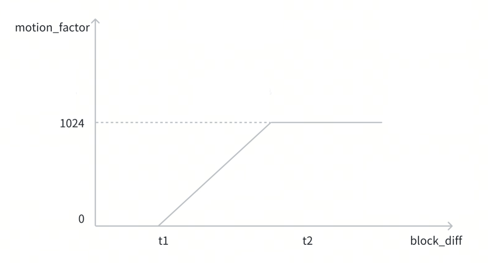
Figure 3.13‑3 3DNR Motion Detection Processing Flowchart

1. Post-processing of Motion Mask

The post-processing step offers two modes, controlled by the parameter “motionSmoothLvl”:

When motion_smooth_Lvl = 1, apply a median filter to the motion mask. This effectively removes noise while preserving edge information, though smoothing is limited.

When motion_smooth_LVL = 0, the post-processing is more complex: first downsample the motion mask to reduce data and eliminate fine noise, then apply median filtering, and finally upsample to restore the original size. This yields significantly smoother motion masks, suitable for scenes requiring strong smoothing.

Users should select the appropriate post-processing mode based on image characteristics and processing needs. The tuning parameters related to motion detection are listed below.

Parameter	Type	Range	Description	Default Value
fixCurveStart	int	[0, 4096]	Curve linearity protection in dark areas, defining the first non-zero X value of the variance stabilization transformation (VST) curve.	256
blsExp[4]	Int[4]	[0, 1048575]	Black level subtraction (BLS) values for images expanded by the noise model.	[0,0,0,0]
vstFactor	double	[1.0, 1000.0]	A factor to control the sigma of the decompose filter. The greater the factor, the larger the decompose sigma.	16
tnrStrength	int	[0, 128]	Output strength of denoised detail. If set to 0, TNR is disabled and the input image is output. If set to 128, TNR is maximized and the TNR result is output.	128
tnrStrength2	int	[0, 128]	Output strength of denoised coarse. If set to 0, TNR is disabled and the input image is output. If set to 128, TNR is maximized and the TNR result is output.	128
filterLen	int	[1, 99]	TNR IIR window size.	1
filterLen2	int	[1, 99]	Motion IIR window size, used for motion history generation.	4
motionSmoothFactor	double	[0.1, 5.0]	Gaussian smooth sigma applied to input images for motion detection. Set to a small value for low ISO and a large value for high ISO.	0.5
rangeH	int	{3, 6}	Width of the motion detection window.	3
sadweight	int	[0, 16]	Weight of the sum of absolute difference (SAD), used to calculate the merged difference as follows: diff = [sad_weight × sad + (16 − sad_weight) × mean_diff]/16 where: · sad_weight is specified by this parameter. · sad is the SAD between the current and reference coarse layers. · mean_diff is the difference between the means of the current and reference coarse layers.	12
diffType	int	{0, 1}	Difference type used for motion detection. 0: merged difference from SAD and mean difference using sadWeight. 1: approximation of squared difference based on the merged difference.	1
sqrDiffFactor	int	[0, 10]	Number of bits shifted to adjust motion difference.	10
noiseLevel	int	[0, 65535]	Motion classifier parameter. If a pixel's motion difference is less than this value, it is classified as static.	32
thrMotionSlope	int	[0, 4095]	Motion classifier parameter. If a pixel's motion difference is greater than the sum of this parameter and noiseLevel, the pixel is classified as 100% moving.	100
tnrLumaCurveX[12]	int[12]	[0, 4095]	Pixel luma curve to define the TNR motion classifier.	[0, 32, 64, 96, 128, 256, 512, 768,1024,1536, 2048, 4095]
tnrLumaCurveY[12]	int[12]	[0, 65535]	Noise level curve to define the TNR motion classifier.	[32, 32, 32, 32, 32, 32, 32, 32, 32, 32, 32, 32]
tnrMotionSlopeY[12]	int[12]	[0, 4095]	Motion slope curve to define the TNR motion classifier.	[100, 100, 100, 100, 100, 100, 100, 100, 100, 100, 100, 100]

Table 3.13‑2 3DNR Motion Detection Tuning Parameters

Motion Mask

A motion mask is a binary image used to mark moving regions in an image or video sequence. It extracts motion information using motion estimation techniques, enabling temporal noise reduction.

The historical frame motion mask detects motion objects in the current frame using past video frames. It analyzes differences between adjacent frames to identify pixel displacements over time, thus locating moving regions in the current frame.

Parameter	Type	Range	Description	Default Value
motionSmoothLvl	int	{0,1}	Smoothing level of the motion mask. Level 0 provides stronger smoothing than level 1.	1

Table 3.13‑3 Motion Mask Tuning Parameters

Motion Dilation

The motion dilation module is designed to stabilize the motion mask by convolving the original image with a motion kernel (also known as a motion template). The shape of the kernel determines the direction and degree of motion blur.

After smoothing the motion mask, horizontal dilation is applied to further optimize image features. This dilation parameter is fixed and preset by firmware, typically requiring no user intervention. Its purpose is to enhance specific structures such as edges and contours, providing clearer features for subsequent image analysis.

Since the dilation parameters are firmware-defined, users do not need to adjust them. However, for special application requirements, reconsideration of these parameters may be necessary.

Parameter	Type	Range	Description	Default Value
dialteH	int	{3,6}	Motion dilation size in horizontal direction.	3

Table 3.13‑4 Motion Dilation Tuning Parameters

NoiseProfile

NoiseProfile reflects the noise level of the module at different brightness levels under various gain settings, estimated by a static calibration tool from input RAW sequences.

The RAW input for calibration should cover flat areas with a certain dynamic range of pixel distribution, better reflecting the module’s inherent noise level under different brightness conditions. The recommended gray card luminance range is 140–160. Refer to the X5-Calibration Tool User Guide for detailed calibration requirements.

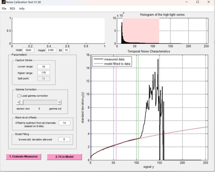
Figure 3.13‑4 NoiseProfile Calibration Diagram

Tuning 3DNR Process

Since 3DNR tuning does not depend on sensor-specific characteristics, tuning starts from the second phase.

Once prerequisites are met, proceed to the tuning process.

Variable	Status/Value
NoiseProfile	Generated by CalibrationTool

Table 3.13‑5 NoiseProfile Calibration Prerequisites

The real-scene setup for 3DNR tuning can be the same as that for 2DNR tuning, including moving objects, ColorChecker, textured objects, color textures, resolution chart, and flat areas. Moving objects are used to assess ghosting artifacts, such as the toy train in Figure 3.13‑5. A metronome is also a good choice for ghosting evaluation.

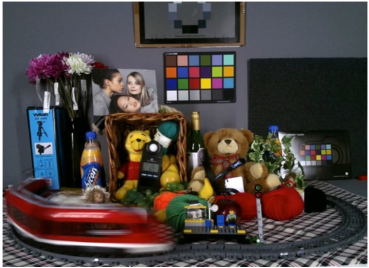
Figure 3.13‑5 Real-scene illustration of 3DNR tuning

Tuning Flow

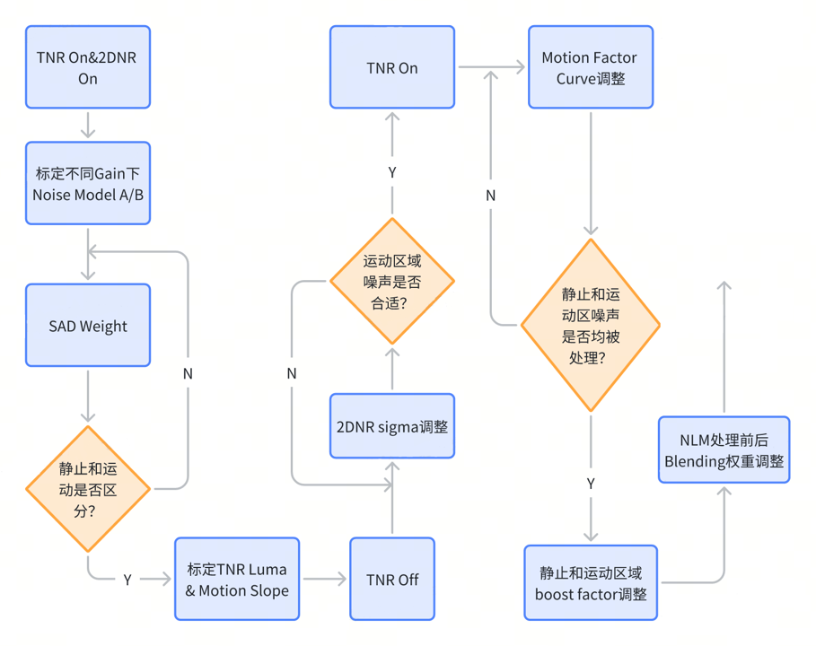
Figure 3.13‑6 3DNR Tuning Flowchart

Detailed 3DNR Tuning Steps

1. Obtain noise_model_a/b through noise calibration.

noise_model_a/b reflects the noise level and trend of raw pixels at different brightness levels under the given exposure. These parameters are used for fitting the TNR noise_level curve and for frequency decomposition in 2DNR.

1. Distinguish motion and static regions.

After determining noise_model_a/b, begin tuning TNR. In high-noise scenes, adjust sad_weight appropriately to rely more on block mean matching, and find a suitable noise_level to separate motion and static regions.

Enable debug dump in configuration and use noise analysis tools to roughly derive two luma-noise level curves from 3DNR debug dumps: one for luma-noise level (tnr luma curve), and one for luma-motion slope (motion slope curve). Based on this, fine-tune tnr luma curve and motion slope curve to better distinguish motion and static regions across different brightness levels. Additionally, tnr factor (filt len) adjusts the weight of historical frames.

Setting tnr_factor to 1 results in slow convergence (~30 frames), reducing static region noise to ~1/30 with smoother output; setting it to a non-1 value (e.g., 10) results in faster convergence (~10 frames), reducing noise to ~1/10 with more residual noise.

1. Adjust 2DNR strength.

Once motion and static regions are reasonably separated, disable TNR and tune 2DNR, focusing on whether 2DNR strength on moving objects is appropriate. It is generally recommended to set detail thr and moving detail thr to 0. Sigma 0, sigma 1, and sigma base represent high, medium, and low frequencies, respectively, typically with sigma0 > sigma1 > sigma base. After finalizing parameters, enable both TNR and 2DNR for joint tuning.

1. Joint tuning of TNR and 2DNR

​ 1) Adjust motion factor curve to apply varying 2DNR strengths from static to motion regions. During this process, motion factor (filt_len2) affects motion joint: increasing motion factor increases the weight of motion history, causing past motion regions to rely more on historical frame information, thus increasing 2DNR strength.

​ 2) The output after NLM is the low-frequency component. Optionally, overlay mid- and high-frequency components. This allows selective enhancement or suppression of texture in static-to-motion regions (limited to detail textures after NLM).

• Below detail threshold: no overlay

• Above detail threshold but below boost detail threshold: overlay without enhancement

• Above boost detail threshold: enhanced overlay

Enhancement coefficient is determined by boot factor.

Static and motion region separation is defined by [anchor0,anchor1]. Two values are selected on the motion joint axis: below anchor0 is static, above anchor1 is motion, and intermediate regions are linearly interpolated. The boost clip parameter limits enhancement—any value exceeding clip is clamped to clip.

Optionally overlay results before and after NLM. After NLM refers to the result after the above processing (b), while before NLM refers to the result after TNR. Overlay ratio can be tuned via nlm strength offset, nlm strength max, and nlm strength slope. For example, if nlm strength offset is 900 and nlm strength max is 1024, then from 0 onward, the post-NLM result accounts for 900/1024, and pre-NLM result accounts for (1024-900)/1024.

From 0 upward, nlm strength increases with a slope until reaching 1024. Overlaying a certain proportion of pre-NLM results introduces slight graininess into otherwise overly smooth areas, which can help alleviate unnatural oily appearance after 2DNR.

Tips:

• 2DNR vstfactor range: [0,1000]; 3DNR vstfactor range: [1,1000];

• Both manual and auto modes in 2DNR include vstfactor; only manual mode in 3DNR includes vstfactor;

• Handling of 3DNR and 2DNR vstfactor:

  • 3DNR auto & 2DNR auto

    The vstfactor calculated by 3DNR auto is passed to 2DNR. If the vstfactor calculated by 2DNR auto is less than 1, use the 3DNR value; otherwise, use the 2DNR value.

  • 3DNR auto & 2DNR manual

    The vstfactor calculated by 3DNR auto is passed to 2DNR, which uses it directly, regardless of the manually set vstfactor in 2DNR.

  • 3DNR manual & 2DNR auto

    2DNR auto uses its own calculated vstfactor, independent of 3DNR parameters.

  • 3DNR manual & 2DNR manual

    2DNR uses its own vstfactor, independent of 3DNR.

Demosaic

Overview

In digital image processing, Demosaic interpolates Bayer data into full RGB color values.

Directional interpolation is applied to different color channels during interpolation to reduce introduced artifacts, while spatial-domain sharpening enhances image clarity.

Tuning Theory

Based on the Bayer matrix, each pixel’s RGB values are reconstructed using isotropic and anisotropic nonlinear color interpolation algorithms for gradient detection, combined with edge-adaptive sharpening to minimize high-frequency noise and suppress color artifacts.

The main goal of Demosaic is to maximize gradient detection accuracy for both isotropic and anisotropic cases. This can be achieved by adjusting gradient detection parameters. The basic processing flow is as follows:

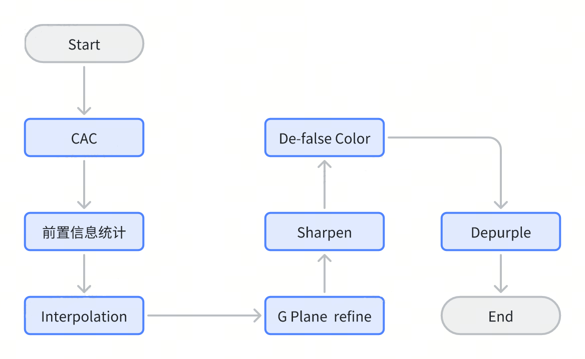
Figure 3.14‑1 Demosaic Processing Flow

Demosaic tuning can be completed in three phases:

• Phase One: No adjustment required.

• Phase Two: Tune key modules such as Interpolation, Sharpen, and De-Purple in a lab environment.

• Phase Three: Fine-tune Demosaic parameters based on real-world scenarios to better adapt to all conditions, mainly involving sharpening parameters that vary with Gain.

CAC

Chromatic aberration occurs when an optical lens fails to focus all wavelengths of light at the same point, primarily due to differing refractive indices for different wavelengths—a common lens defect. Typically, chromatic aberration is more pronounced farther from the image center, often appearing as different colors along object edges. CAC scales the R and B planes relative to the G plane to align all three channels, with scaling direction and strength obtained through calibration.

CAC parameters are highly module-specific. CAC correction coefficients are generated via CalibrationTool. When importing objective calibration-generated JSON or XML files through Vtuner, the tool automatically writes the CA calibration parameters into the DMSC CAC section. The table below describes each parameter in the ISP pipeline’s CAC module. Modification is not recommended; use tool-calibrated values as reference.

Parameter	Type	Range	Description	Default Value
cacEnable	bool	{true, false}	Enable the CAC module in demosaic	false
aBlue	float	[-16,15.9375]	Linear parameters for radial shift calculation in blue channel	0
aRed	float	[-16,15.9375]	Linear parameters for radial shift calculation in red channel	0
bBlue	float	[-16,15.9375]	Square parameters for radial shift calculation in blue channel	0
bRed	float	[-16,15.9375]	Square parameters for radial shift calculation in red channel	0
cBlue	float	[-16,15.9375]	Cubical parameters for radial shift calculation in blue channel	0
cRed	float	[-16,15.9375]	Cubical parameters for radial shift calculation in red channel	0
centerHoffs	int	[0,image_width/2]	Horizontal distance between image and optical center in pixels	0
centerVoffs	int	[0,image_height/2]	Vertical distance between image and optical center in pixels	0

Table 3.14‑1 CAC Calibration Correction Parameters

Chromatic aberration is typically more noticeable at image corners than at the center. Generally, its intensity depends on the distance from the optical image center. The algorithm corrects this via polynomial operations that dynamically adjust color distribution as a function of radius from the optical center. It uses a 9-bit two’s complement integer with 4 fractional bits, effective range [-16, 15.9375]. For example, B channel correction is calculated as:

This polynomial allows setting linear, quadratic, and cubic terms to fit the observed chromatic aberration function. Correction should be performed using appropriate computational tools along with test images generated from the sensor model to be corrected.

If the lens system does not perfectly align with the sensor array, the image center may deviate from the chromatic aberration center. This offset can be corrected by setting the following registers:

• h_𝑐𝑜𝑢𝑛𝑡_𝑠𝑡𝑎𝑟𝑡[bits 12:0]

• 𝑣_𝑐𝑜𝑢𝑛𝑡_𝑠𝑡𝑎𝑟𝑡[bits 28:16]

Calculation method:

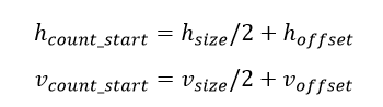
Where

• $h_{size}$ is the number of horizontal pixels

• $v_{size}$ is the number of vertical pixels

• $h_{offset}$ is the horizontal pixel distance between image center and optical center

• $v_{offset}$ is the vertical pixel distance between image center and optical center

Maximum distance from image center:

$$dist_ max = \sqrt{{h_ count_ max}^{2} + {v_ count_ max}^{2}}$$

$h_ count_ max$ and $v_ count_ max$ are the maximum pixel counts in horizontal and vertical directions, respectively.

The relationship among these parameters is illustrated in Figure 3.14‑2.

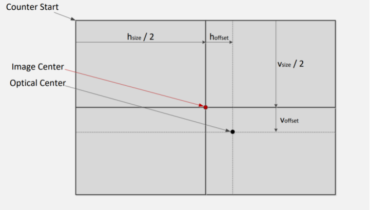
Figure 3.14‑2 Relationship Between Image Center and Optical Center

Interpolation

During interpolation in the Demosaic module, the input image undergoes gradient calculation, separation of edges and flat areas, direction judgment, corner detection, etc. Based on all these results, the input Bayer image is interpolated into RGB. Typically, interpolation module parameters do not require adjustment and should remain at default values.

Parameter	Type	Range	Description	Default Value
dmsc3Enable	bool	{false , true}	DMSC enable/disable	true
granThMin	int	[0,4095]	During interpolation, flat area (mean value interpolation) upper_bound/lower_bound threshold determination: 1. lower_bound refers to darkest area. 2. upper_bound refers to brightest area. ==> each pixel calculates brightness within 5x5 window and calculates threshold adaptively	4
granThMax	int	[0,4095]	20
diffColorCoef	int	[0,128]	1. weighted fusion ratio for "cross channel difference" wt 2. weighted fusion ratio for "inner channel difference" 128-wt	128
adptCoefMode	int	[0,3]	self-adaptive model for different channel switch: 0: self-adaptive mode disable, use dmsc3_diffColor_coef 1: self-adaptive mode for pixels in R&B channel 2: self-adaptive mode for pixels in Gr&Gb channel 3: self-adaptive mode applied to all selected pixels	3
adptCoefThLow	int	[0,255]	with coef enable: local average color difference and stability ==> cross channel difference use "dmsc3_adpt_coef_min" to determine direction when average&stability is under this threshold ==> cross channel difference use "dmsc3_adpt_coef_max" to determine direction when average&stability is beyond (th_low + (1 << th_shift)) ==> (1<<shift) indicates the transition area from "dmsc3_adpt_coef_min" to "dmsc3_adpt_coef_max"	24
adptCoefThShift	int	[0,8]	6
adptCoefMin	int	[0, 128]	minimum/maximum coefficient involved in direction determination for cross channel difference with AdptCoefMode enable	0
adptCoefMax	int	[0, 128]	128
interpCornerEn	bool	{false , true}	corner rough selecting enable/disable	true
interpDirStrength[4]	int[4]	[0,256]	horizontal/vertical rough selecting; h/v directional end selecting; h/v 2nd round selecting; h/v 3rd round selecting	[32,64,32,16]
interpLargeStr[2]	int[2]	[0,16]	directional weighted fusion for large area and small area corresponding to 2nd/3rd h/v directional selecting.	[12,4]
dir0InterpType	int	[0,3]	For non-ISO and direction unclear pixel, choose interpolation method: 0: mean interpolation method in flatter area like ISO point; 1~3: use different method based on surrounding pixels;	0
cornerLowTh	int	[0,4095]	threshold for directional interpolation, lower bound threshold refers to directional average: (cornerLowTh + (1 << cornerShift)): threshold for directional interpolation, upper bound threshold refers to weighted directional similarity: transition area; larger value tends to use mean interpolation, smaller value tends to use non-mean interpolation	1024
cornerShift	int	[0,12]	6
declineEn	bool	{false , true}	high brightness compression during RB interpolation: determine if filter out row/column with high brightness	true
highlightControlTh	int	[0,4095]	Threshold for high brightness determination	1024
highlightControlShift	int	[0,9]	Width for transition area: (1 << highlightControlShift)	6
deburstMode	int	[0,3]	No channel selected for deburst 1: Deburst for g channel during interpolation 2: Deburst for rb channel during interpolation 3: Deburst for rb and g channel during interpolation	3
pureGWeight	int	[0,16]	During G interpolation in uneven area use "non color diff interpolation result" (weight) and "color diff interpolation result" in flat area (16-weight)	0
pureRBWeight	int	[0,16]	During R/B interpolation in uneven area use "non color diff interpolation result" (weight) and "color diff interpolation result" in flat area (16-weight)	0
pureGWeightISO	int	[0,16]	During G interpolation in flat area use "non color diff interpolation result" (weight) and "color diff interpolation result" in flat area (16-weight);	0
pureRBWeightISO	int	[0,16]	During R/B interpolation in flat area use "non color diff interpolation result" (weight) and "color diff interpolation result" in flat area (16-weight)	0
demoireRefineGEn API	bool	{false , true}	correct G value based on interpolation direction of surrounding pixels.	true
refineGTh	int	[0,4095]	refine G focus on interpolated G value. If difference of R and B is larger than setting, start the correction.	100
DeFalseColorEn API	bool	{false , true}	defalse color enable/disable (open by default and recommended)	true

Table 3.14‑2 DMSC Interpolation Tuning Parameters

Sharpen

The Sharpen sub-function in Demosaic enhances edges and improves clarity. It supports frequency band separation, enabling sharpening enhancement in different frequency bands. The Sharpen module decomposes the input image into high, medium, and low frequency bands, each processed in three stages.

The entire Sharpen processing flow is shown below:

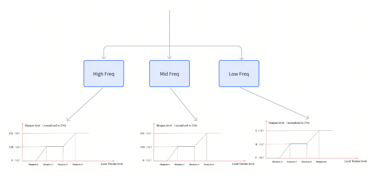
Figure 3.14‑2 Demosaic Sharpen Processing Flow

Detailed descriptions of Demosaic Sharpen module parameters are as follows.

Parameter	Type	Range	Description	Default Value
dmscSharpenEnable	bool	{false , true}	true: enables the sharpen function in demosaic. false: disables the sharpen function in demosaic.	true
dmscSharpenCurve0T1	int	[0,2047]	The texture value threshold T1. For the curve illustration, see Figure 3.14-3.	32
dmscSharpenCurve0T2Shift	int	[0,11]	The shift to T1 which determines the texture value threshold T2 as follows: T2 = T1 + 2t2_shift	6
dmscSharpenCurve0T3	int	[0,2047]	The texture value threshold T3	122
dmscSharpenCurve0T4Shift	int	[0,11]	The shift to T3 which determines the texture value threshold T4 as follows: T4 = T3 + 2t4_shift	6
dmscSharpenCurve0R1	int	[0,256]	The sharpen levels R1, R2, and R3. The larger the longitudinal axis, the stronger the texture sharpening.	0
dmscSharpenCurve0R2	int	[0,256]	100
dmscSharpenCurve0R3	int	[0,256]	126
dmscSharpenCurve1T1	int	[0,2047]	The texture value threshold T1. For the curve illustration, see Figure 3.14-3.	8
dmscSharpenCurve1T2Shift	int	[0,11]	The shift to T1 which determines the texture value threshold T2 as follows: T2 = T1 + 2t2_shift	5
dmscSharpenCurve1T3	int	[0,2047]	The texture value threshold T3	64
dmscSharpenCurve1T4Shift	int	[0,11]	The shift to T3 which determines the texture value threshold T4 as follows: T4 = T3 + 2t4_shift	5
dmscSharpenCurve1R1	int	[0,256]	The sharpen levels R1, R2, and R3. The larger the longitudinal axis, the stronger the texture sharpening.	0
dmscSharpenCurve1R2	int	[0,256]	126
dmscSharpenCurve1R3	int	[0,256]	168
dmscSharpenCurve2T1	int	[0,2047]	The texture value threshold T1. For the curve illustration, see Figure 3.14-3.	0
dmscSharpenCurve2T2Shift	int	[0,11]	The shift to T1 which determines the texture value threshold T2 as follows: T2 = T1 + 2t2_shift	6
dmscSharpenCurve2T3	int	[0,2047]	The texture value threshold T3.	72
dmscSharpenCurve2T4Shift	int	[0,11]	The shift to T3 which determines the texture value threshold T4 as follows: T4 = T3 + 2t4_shift	67
dmscSharpenCurve2R1	int	[0,256]	The sharpen levels R1, R2, and R3. The larger the longitudinal axis, the stronger the texture sharpening.	0
dmscSharpenCurve2R2	int	[0,256]	The sharpen levels R1, R2, and R3. The larger the longitudinal axis, the stronger the texture sharpening.	152
dmscSharpenCurve2R3	int	[0,256]	The sharpen levels R1, R2, and R3. The larger the longitudinal axis, the stronger the texture sharpening.	200

Table 3.14‑3 DMSC Sharpen Tuning Parameters

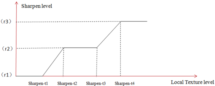
Figure 3.14‑3 Demosaic Sharpen Level Illustration

As shown in the figure above, the larger the Y-axis value, the stronger the texture sharpening.

Larger t-series values (or smaller r-series values) shift the curve rightward (downward), indicating lower overall sharpening.

• Gradient values below t: sharpen value set to r1;

• Gradient values between t2 and t3: sharpen value set to r2;

• Gradient values above t4: sharpen value set to r3; other regions use linear interpolation to determine sharpen value.

Black&White Edge Control

Black-and-white edge sharpening typically detects edge regions in the image and applies a sharpening filter to enhance edge contrast. This makes object boundaries clearer, improving image clarity and resolution.

Note that excessive sharpening may introduce noise or artifacts, so adjustments should be made carefully based on specific conditions to achieve optimal results.

Separate factors for black and white can be set to control enhancement strength.

Separate clips for black and white can be set to limit the maximum sharpening strength.

Parameter	Type	Range	Description	Default Value
dmscSharpenFactor	int[6]	[0,511]	Enhancement ratios for high, middle, and low frequencies on brighter and darker sides.	[100,100,200,200,300,300]
dmscSharpenClip	int[6]	[0,2047]	Enhancement clip values for high, middle, and low frequencies on brighter and darker sides.	[20,30,30,30,30,40]

Table 3.14‑4 DMSC Sharpen Tuning Parameters

Sharpen Line

The Line Sharpen function mainly distinguishes edges and textures from flat areas in the image, applying a sharpening filter to enhance edge contrast and detail. This makes object boundaries clearer and texture details richer, improving image clarity and resolution performance.

Parameter	Type	Range	Description	Default Value
dmscSharpenLineEnable	bool	{true,false}	true: enables the line sharpen function in demosaic. false: disables the line sharpen function in demosaic. Setting this parameter to false is recommended.	false
dmscSharpenLineStrength	int	[0,4095]	The weight of the sharpen_line image for merging into the output image.	8
dmscSharpenLineThr	int	[0,2047]1	The line detection threshold T1. For the curve illustration, see Figure 3.14-4.	24
dmscSharpenLineThrShift1	int	[0,11]	The shift to T1 which determines the line detection threshold T2 as follows: T2 = T1 + 2t2_shift	3
dmscSharpenLineR1	int	[0,256]	The sharpen levels R1 and R2. The larger the longitudinal axis, the stronger the texture sharpening.	0
dmscSharpenLineR2	int	[0,256]	The sharpen levels R1 and R2. The larger the longitudinal axis, the stronger the texture sharpening.	256

Table 3.14‑5 DMSC Sharpen Line Tuning Parameters

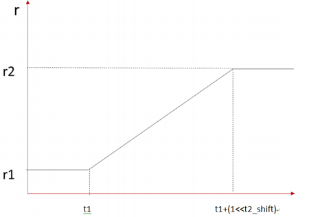
Figure 3.14‑4 Sharpen for t1 and t2

As shown in Figure 3.14‑4, the larger the vertical axis value, the more the sharpening result approaches directional (horizontal or vertical) enhancement. At the same time, more points may break apart, which could lead to artifacts in high-frequency details. The basic effect is to smooth lines or textures in vertical or horizontal directions. The default setting is to disable sharpening.

De-Purple

The De-Purple function aims to identify purple fringes in high-contrast regions of the image. Using a color correction algorithm, it dynamically adjusts the strength of purple fringe removal based on the color distribution in the image and corrects these purple edges by adjusting saturation. This function detects high-contrast edge gradients within a defined region by setting luminance thresholds for Cb (blue difference) and Cr (red difference). For regions identified as purple fringes, the system applies desaturation processing to eliminate unwanted purple edges, thereby improving image quality. This method is highly effective in reducing chromatic aberration generated by imaging sensors, especially under conditions of extremely high edge contrast.

Below is the processing flowchart of the De-Purple module:

Figure 3.14‑5 Demosaic DePurple Processing Flowchart

Key parameters of the purple fringe removal module are as follows:

Parameter	Type	Range	Description	Default Value
dmscDepurpleEnable	bool	{true, false}	true: enables the depurple function in demosaic. false: disables the depurple function in demosaic.	false
gradControl	int	[0,1]	0: disables gradient protection that is integrated in demosaic v3. 1: enables gradient protection that is integrated in demosaic v3.	1
protectThLow	int	[0,255]	The upper and lower thresholds of gradient protection. Lower threshold: protectThLow Upper threshold: protectThLow + (1 << protectShift)	16
protectShift	int	[0,8]	The upper and lower thresholds of gradient protection. Lower threshold: protectThLow Upper threshold: protectThLow + (1 << protectShift)	5
dmscDepurpleSatShrink	int	[0,8]	The desaturation strength. A greater value leads to a stronger desaturation strength.	8
dmscDepurpleCbcrMode	int	{0, 1, 2, 3}	The desaturation mode on Cb/Cr channels. 0: depurple disabled. 1: Cr channel depurple. 2: Cb channel depurple. 3: Cr/Cb channel depurple.	3
dmscDepurpleThr	int	[0, 255]	The threshold to judge purple areas.	40
cbLowth[0]	int	[0, 255]	The upper and lower bounds for Cr/Cr color region 1.	132
cbHighth[0]	int	[0, 255]	The upper and lower bounds for Cr/Cr color region 1.	220
crLowth[0]	int	[0, 255]	The upper and lower bounds for Cr/Cr color region 1.	112
crHighth[0]	int	[0, 255]	The upper and lower bounds for Cr/Cr color region 1.	200
cbLowth[1]	int	[0, 255]	The upper and lower bounds for Cr/Cr color region 2	96
cbHighth[1]	int	[0, 255]	The upper and lower bounds for Cr/Cr color region 2	122
crLowth[1]	int	[0, 255]	The upper and lower bounds for Cr/Cr color region 2	82
crHighth[1]	int	[0, 255]	The upper and lower bounds for Cr/Cr color region 2	118

Table 3.14‑6 DMSC Depurple Tuning Parameters

dmscDepurpleThr is the threshold used to detect purple values in the image. If the purple value exceeds the threshold, DMSC will perform desaturation and color compensation processing. If the purple value is below the threshold, DMSC performs no operation. The smaller the threshold is set, the more purple edges will be detected. It is recommended to set this value greater than or equal to 40.

dmscDepurpleSatShrink directly desaturates points in purple regions. The maximum value is 8, which forces complete desaturation and converts the region to grayscale when purple is detected. The ideal value is 0 or slightly greater than 0.

Figure 3.14‑6 Demosaic Depurple Function Illustration

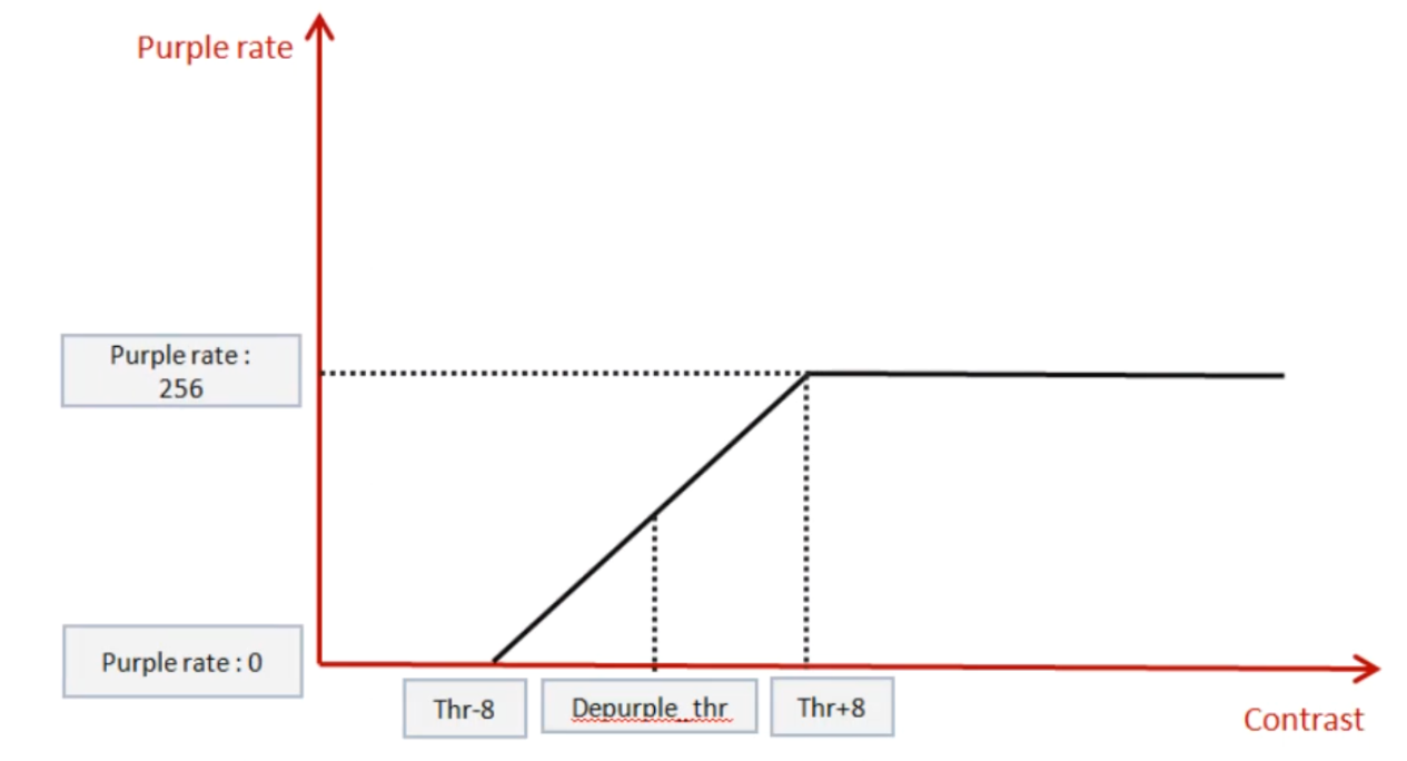
The smaller the threshold value, the more pixels will be considered as purple fringes. Since the current detection only identifies edges without analyzing color, the “desaturation” function should be used with caution.

DeFalse Color

In demosaic processing, de-false color is used to eliminate color distortions caused by the CFA pattern and interpolation algorithms. These distortions typically appear as colored stripes or spots near high-contrast edges, especially in detail-rich areas.

The false color removal algorithm works by detecting regions in the image where false colors may occur and applying local color correction to these regions. This usually involves analyzing color differences between adjacent pixels and smoothing suspected false color pixels to reduce color distortion.

Parameter	Type	Range	Description	Default Value
DeFalseColorEn API	bool	{true, false}	defalse color enable/disable (open by default and recommended)	true
ColorStr	int	[0,128]	defalse color strength (default and fixed 128)	128
cbCrClassTh	int	[0,7]	threshold for median based classification (5 or 6 recommended)	5
grayProtectStr	int	[0,128]	If new_cbcr has higher saturation than old_cbcr, activate this function higher value refers to heavier weighted old_cbcr	0

Table 3.14‑7 DMSC DeFalse Color Tuning Parameters

Demoire

Parameters related to the demoire module are as follows:

Parameter	Type	Range	Description	Default Value
demoireRefineGEn API	bool	{true, false}	correct G value based on interpolation direction of surrounding pixels.	true
refineGTh	int	[0,4095]	refine G focus on interpolated G value. If difference of R and B is larger than setting, start the correction.	100

Table 3.14‑8 DMSC Demoire Tuning Parameters

Tuning during Demosaic phase two

Because initial tuning uses .RAW images, the Demosaic module is not adjusted until the second phase. Adjustment can only begin after the following prerequisites listed in the table below are met:

Prerequisite	Status / value
Black level	Tuned
Noise profile	Derived
Green equalization	Tuned
Defective pixel correction	Tuned
2DNR	Tuned and enabled
3DNR	Tuned and enabled

Table 3.14‑9 Demosaic Prerequisites

Tuning Process —— Sharpening

The sharpening module in Demosaic is related to edges and textures in the image. It only sharpens detected edges and textures, leaving flat areas unprocessed. The purpose is to properly balance image sharpness and artifacts.

Edge and texture detection can be achieved by setting gradient variation values via layerT1, layerT2Shift, layer0T3, and layerT4Shift. T1, T2, T3, and T4 represent increasing levels of texture detail richness. Edge and texture enhancement can be individually controlled through layerR1, layerR2, and layerR3, which set sharpening strength for different texture-rich regions.

Note: 1. Although Sharpen can improve objective performance metrics, it may degrade subjective image quality. Artifacts such as “haloing” and noise are typically caused by over-sharpening.

2. To apply different sharpening strengths for textures and edges, adjust the sharpenCurveIndex value to modify sharpening strength across different frequency bands (high, medium, low) under varying texture conditions.

This process requires extensive subjective and objective evaluation during image quality testing. The tuning process should use a large number of images captured under different lighting conditions and scenes. Begin tuning from the minimum Gain value before adjusting other system Gain parameters.

Sharpen tuning flowchart:

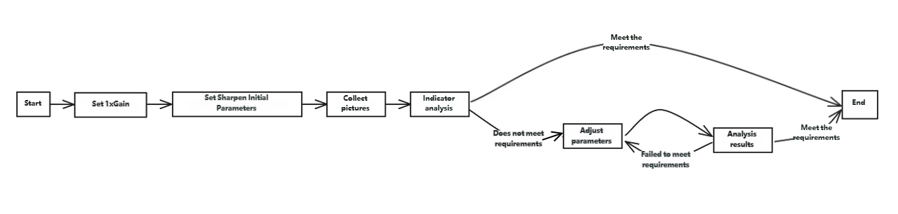
Figure 3.14‑7 Demosaic Sharpen Tuning Flowchart

Sharpness Adjustment Steps

1. Set the Total gain value to 1x.

2. Set initial Sharpen parameters. It is recommended to use default values or those used in previous projects.

3. Properly place the resolution chart and adjust the environment to capture images.

4. Metric analysis.

 

1. Open Imatest and analyze the captured image using the SFR module. Specific metric requirements depend on customer needs, but MTF50 values below or close to 0.5 (cycles/pixel) and overshoot below or close to 10% can serve as baseline tuning references. Both values can be obtained from Imatest’s SFR module output.

2. In the analysis results, MTF50 and overshoot correspond to the Edge profile and SFR (MTF) result items, respectively.

 

1. If requirements are not met, adjust the values of layerR1, layerR2, and layerR3 within a range of +/-5, analyze the results, and repeat until requirements are satisfied.

Additional tuning information:

If the final resolution target is not achieved or visible artifacts exist in the image, optimization of tuning parameters is required. Below are methods to achieve this:

• Disable the Dynamic Pixel Correction (DPCC) module via VTunerClient to check whether this module introduces artifacts. If artifacts disappear, re-tune DPCC parameters and evaluate their impact on other modules after each adjustment.

• Disable the GE module via VTunerClient to check whether Green Equalization (GE) introduces artifacts. If artifacts disappear, re-adjust the threshold value.

• Check whether the image appears blurred due to excessive noise reduction strength, especially in well-lit conditions.

• Understand the limitations of the camera system, as the sensor and optical components used affect the overall system resolution.

Fine tuning demosaic phase three

Tuning the modulation table across the system’s Total Gain range. The prerequisites are as follows:

Prerequisite	Status / value
Phase 2 Tuning	Completed
2DNR	Tuned
3DNR	Tuned
EE	Disabled

Table 3.14-10 Sharpen Prerequisites

For all Gain values within the Total Gain range, repeat steps 1–4 of the Sharpening tuning process from phase two, and fill the corrected values into the corresponding LUT table for each Gain.

Color Correction Matrix (CCM)

Overview

The CCM module corrects and adjusts colors according to customer preferences. It modifies the chrominance values of the image to match standard color space values. This is achieved by capturing a Colorchecker chart and using all color patches along with their reference chrominance values. In most cases, standard colors do not provide optimal image quality. Based on application or customer preferences, these values are calibrated to better meet product requirements.

The adjustment process allows control over overall hue and saturation, which will be introduced as follows:

• Phase one — Adjust CCM using .RAW images in the Calibration Tool.

• Phase two — Adjust CCM using .RGB images under laboratory conditions via the Calibration Tool.

• Phase three — Fine-tune CCM parameters based on gain to suit all scenarios.

Tuning Theory

The CCM module in the ISP is used to correct crosstalk effects and color space shifts within the camera sensor.

The CCM module performs a standard RGB to R’G’B’ color space transformation to compensate for crosstalk between color components in the image sensor. Additionally, color space and saturation can be corrected through appropriate matrix coefficients.

Thus, the module can correct each pixel value via matrix operations as follows:

CCM-related tuning parameters are as follows:

Parameter	Type	Range	Description	Default Value
enable	bool	{true,false}	Whether to enable CCM	true
ccMatrix[9]	float[3][3]	13-bit: [-2048/128, 2047/128] 12-bit: [-8, 7.992]	Gain for each channel	[[1.0, 0, 0], [0, 1.0, 0], [0, 0, 1.0]]
ccOffset[3]	float[3]	[-2047, 2047]	Offset for each channel	[0.0, 0.0, 0.0]

Table 3.15‑1 CCM Static Calibration Parameters

Tuning during phase one

Prerequisites

Prerequisite	Status / value
Black level	Tuned
Lens shading	Tuned
Initial gamma	Tuned
CNR	Disabled
Manual exposure	−0.25 \< exposure error \< 0.25 (f-stops). This can be verified through Imatest. Avoid clipping of patch 19 from the ColorChecker chart

Table 3.15‑2 CCM Tuning Prerequisites

Tuning Process

In this initial adjustment phase, perfect CCM values are not expected. Follow the CCM calibration steps in the X5-Calibration Tool User Guide to obtain CCM values under different color temperatures. The most critical adjustments occur in phase two and phase three.

Tuning during phase two

Prerequisites

Prerequisite	Status / value
Phase one prerequisites	Complete
AWB	Tuned
gamma	Disabled
AE	−0.25 \< exposure error \< 0.25 (f-stops). This can be verified through Imatest.

Table 3.15‑3 CCM Phase Two Prerequisites

Tuning Process

Before tuning CCM in phase two, use Imatest’s Colorcheck module to verify exposure error. If the exposure error is not within the range specified in Table 3.15‑2, readjust the AE_target parameter to correct exposure. Repeat this process until exposure is accurate.

The adjustment in phase two is very similar to phase one. Adjust the calibrated CCM values under different color temperatures according to specific image requirements to achieve the desired visual style.

Fine tuning phase three

Phase three includes two main parts: updating calibration parameters and saturation modulation. The first focuses on reflecting changes in prior module parameters. The second defines gain-dependent CCM, aiming to provide better noise control under higher gain or lower illumination conditions.

Note: The trade-off between color accuracy and noise visibility must be carefully considered at each gain level. Typically, the goal is to provide maximum saturation without introducing unnecessary noise. Always consider customer requirements or intended applications.

Extensive fine-tuning in phase three is often required due to changes in parameters of modules on which CCM depends (e.g., gamma). This may necessitate re-tuning and updating CCM based on results from phase two.

Saturation modulation

As illumination gradually decreases, if certain adjustments to saturation at different illuminance levels are needed to reduce introduced color noise, the percentage of saturation can be adjusted under different color temperatures during CCM calibration. This generates multiple sets of CCM matrices with different target saturation levels. These can be generated during calibration parameter generation. In practical tuning applications, saturation reduction processing based on Gain and CCT (two-dimensional) can be achieved by changing the corresponding Gain value in the JSON configuration file.

Gamma Correction

Overview

The Gamma module performs nonlinear brightness transformation on the image to match output devices, primarily used to adjust contrast.

The RGB Gamma module is used to create gamma pre-corrected images commonly used in video processing. A gamma value of 1.0 indicates a linear relationship, where output values are directly proportional to input values. Most displays and image formats use a gamma value of approximately 2.2, with a linear segment at the beginning of the gamma curve, providing brightness levels that better match perceptual uniformity.

Values between nodes in the Gamma table are generated using linear interpolation. The tuning process is as follows:

• Phase one: Use the Calibration Tool to tune in a laboratory environment; tuning results should cover most scenarios.

• Phase two: Adjust Gamma according to AE_target to improve contrast.

• Phase three: Fine-tune Gamma to make contrast suitable for all scenarios.

Tuning theory

The R, G, and B channels use different Gamma LUTs, each consisting of 64 uniformly spaced nodes, with linear interpolation between nodes. Each data point is a 10-bit unsigned type, so gamma[0]=0, gamma[64]=1023. These node values define the gamma correction curve.

When standard is set to true, setting standardVal directly generates the corresponding gamma curve. When standard is set to false, the standardVal parameter is grayed out and standard gamma curves cannot be obtained, but users can manually drag curve anchors or modify LUT values to adjust the Y-axis values of the gamma curve for custom curves.

By default, the X-axis of the Gamma curve consists of uniformly spaced nodes. To customize the X-axis node distribution, set userCurveX to true and adjust the curvePx values to modify X-axis node positions. The modified X-axis node positions are given by:

Where

Table 3.16-1 lists the tuning parameters of the Gamma module:

Parameter	Type	Range	Description	Default Value
enable	bool	{true,false}	Enable/disable the Gamma module	true
standard	bool	{true,false}	If false, use the customized curve	true
standardVal	float	[1,4]	Generate uniform curve with gamma formula	2.2
curve[64]	Int[64]	[0,1023]	Gamma curve.	[155, 212, 255, 290, 321, 349, 374, 398, 419, 440, 460, 478, 496, 513, 529, 545, 560, 575, 589, 603, 617, 630, 643, 655, 667, 679, 691, 703, 714, 725, 736, 747, 757, 767, 778, 788, 798, 807, 817, 826, 836, 845, 854, 863, 872, 881, 889, 898, 906, 915, 923, 931, 939, 947, 955, 963, 971, 978, 986, 994, 1001, 1008, 1016, 1023]
userCurveX	bool	{true,false}	Use the manual/inline value true: Use the manual value false: Use the inline value	false
curvePx[64]	Int[64]	[0,12]	The x point of manual curve	[0, 0, 0, …,0, 0, 0]

Table 3.16‑1 Gamma Tuning Parameters

Tuning during phase one

Typically, initial Gamma tuning only requires setting one initial Gamma Curve, saving it, and proceeding to other modules. Gamma should be re-evaluated in phase two during AE module tuning to determine if further adjustment is needed to enhance contrast.

In this initial adjustment phase, refer to the CCM calibration instructions in the X5-Calibration Tool User Guide to select a Gamma curve or use an existing Gamma Curve from a prior project as the reference curve.

Tuning during phase three

In subsequent real-scene adaptation, dynamically adjust the Gamma curve based on actual scene requirements to meet image contrast requirements. Adjusting the Gamma Curve may cause some fluctuation in color metrics. If specific color accuracy requirements exist, color performance must be re-measured after modifying the Gamma Curve, and CCM may need to be recalibrated.

The Gamma module can use different Gamma curves for different Gain settings. In practical applications, set corresponding Gamma curves according to actual scene needs, ensuring relatively smooth transitions between Gamma curves of adjacent Gain levels.

Edge Enhancement

Overview

Edge Enhancement (EE) improves the edge contrast of objects in the image.

The main purpose of the EE algorithm is to detect as many object edges as possible through edge detection. The edge detection result describes the sharpness level of different edges. Edges can be smoothly enhanced based on different sharpness levels.

Tuning Theory

A brief overview of the tuning process is as follows:

• Phase one: No adjustment required.

• Phase two: Adjust EE enhancement parameters under laboratory conditions for most scenarios.

• Phase three: No adjustment required unless prior tuning parameters or modules on which EE depends produce poor image quality.

The complete processing flowchart of the EE module is shown below:

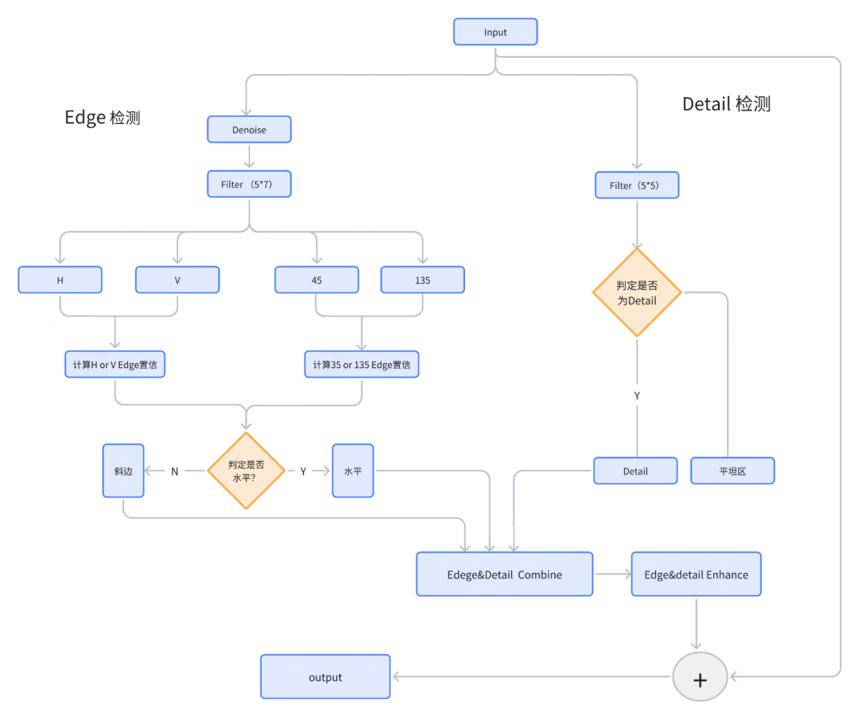
Figure 3.17‑1 EE Processing Flowchart

Edge Enhanced

Edge Enhancement (EE) is used to improve object edges. High-frequency information is separated into edges and details, allowing independent control of edge and detail sharpening styles. Isotropic filters are used for details to achieve a more natural sharpening style, while anisotropic filters are used for edges to achieve sharper edges.

This module includes three main parts:

1. Enhancement of the Y channel at object edges. This part improves image clarity without increasing noise.

2. Reduction of saturation in the UV channels at object edges. This part reduces color saturation at object edges. As color saturation decreases, chromatic aberration and color fringing are significantly reduced.

3. Enhancement of image contrast. This module can improve local or overall image contrast by adjusting contrast across different brightness levels.

Enhancement strength is fully enabled when lighting in the image is exceptionally good (sensor analog gain is very low), such as in outdoor scenes or bright rooms. Edge enhancement strength is reduced under low-light conditions (high sensor analog gain).

Parameter	Type	Range	Description	Default Value
eeEnable	bool	{true,false}	true: enables edge enhancement (EE). false: disables EE.	true
yuvDomain	bool	{true,false}	true: processes EE in the YUV domain. false: processes EE in the RGB domain.	false
strength	int	[0, 128]	The EE strength, which determines the degree to which the enhanced result is merged back to the input image. If this parameter is set to 128, it indicates that 100% enhanced result is used.	128
srcStrengthskin	int	[0, 256]	The low-frequency fusion by original Y value and low-pass filter result. This parameter affects only the detected skin zones.	256
gradTh[2]	int	[0,1024]	The distinguish threshold for edge and noise, and the distinguish threshold for edge and details.	[8,12]
edgeNrLvl	int	[0,5]	The noise reduction level. Value 0 indicates the lowest level and value 5 indicate the highest level.	3
edgeScaler	int	[0,32]	The scaler control for edge detection results.	4
edgeUseAuxiDir	int	[0,1]	Indicates whether to take the auxiliary direction into consideration for edge strength generation during edge detection. 0: does not take the auxiliary direction into consideration. 1: takes the auxiliary direction into consideration.	1
detailLvl	int	[0,7]	The detail level, which determines the sharpen style. A smaller value leads to more fine-grained enhancement.	5
detailScaler	int	[0,32]	The scaler control for texture/detail detection results.	8
detailPreEnhanceStr	int	[0,256]	The texture/detail strength. A greater value leads to a higher detail level.	16

Table 3.17‑1 EE Tuning Parameters

gradTh Parameter Description:

Differentiates edges from noise based on image gradient information.

Smaller threshold values result in more complete edge detection but increased noise. Larger values result in fewer detected edges—potentially detecting only larger edges while suppressing weaker edges and noise.

EE Sharpen

Parameters related to edge sharpening are as follows:

Parameter	Type	Range	Description	Default Value
sharpCurveLvl	int	[0,7]	The enhancement curve selection. 0 to 6: Detail mode influence is increased as the value increases. 7: The former part is the same as curve 3 and the later part enhances the compression of strong edge.	3
sharpGain[2]	int	[0,1024]	The strength of the brighter side and that of the darker side in non-skin areas	[100,122]
sharpGainUv	int	[0,255]	The UV sharpen strength near edges.	0
sharpLimitEn	bool	{true,false}	true: enables sharpen extreme value constrain. false: disables sharpen extreme value constrain.	true
sharpLimitType	int	[0,2]	The type of sharpen extreme value control. 1: High-frequency enhancement is within a certain ratio of the original value. 2: High-frequency enhancement is within a certain ratio of the local original value. 3: High-frequency enhancement is within a certain ratio of the adjusted local original value.The default value 2 is recommended.	2
sharpLimit[2]	int	[0,512]	The upper limit and lower limit of the range within which the difference after highfrequency enhancement is constrained. You can determine the range by the local brightest and darkest and the pre-set ratio.	[90,118]
hfMergeCurve[4]	Int[4]	Element 1: [0, 1024] Element 2: [0, 10] Element 3: [0, 1024] Element 4: [0, 10]	The fusion cure of noise, texture, and edge. Element 1: The threshold T1. Element 2: The shift to T1 which determines the threshold T2 as follows: T2 = T1 + 2t2_shift Element 3: The threshold T3. Element 4: The shift to T3 which determines the threshold T4 as follows: T4 = T3 + 2t4_shift	[4,4,24,8]

Table 3.17‑2 EE Sharpen Tuning Parameters

sharpCurveLvl Parameter Description:

When this field is set to a value between [0, 6], a larger value results in greater enhancement of the detail portion.

When this field is set to 7, the enhancement curve matches the first half of curve 3, while the second half suppresses strong edge enhancement.

Typically, this field is set to 3 or 7. Increase this value when enhancing details or strengthening weak edges. Decrease this value when suppressing noise in flat areas.

sharpLimitType Parameter Description:

0: The difference from high-frequency enhancement does not exceed a certain ratio of the original value (set by change_up/down).

1: The difference from high-frequency enhancement does not exceed a certain ratio of the local brightest/darkest value (set by change_up/down).

2: The difference from high-frequency enhancement does not exceed a certain ratio of the adjusted local brightest/darkest value (adjusted globally and set by change_up/down).

hfMergeCurve Parameter Description:

Edges and details divide the image into two parts: edge regions and non-edge regions. Edge regions contain edges and contours in the image, while non-edge regions contain smooth areas and details. These two regions are processed separately and then merged.

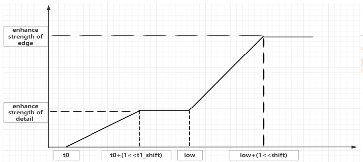
Figure 3.17‑2 EE Edge&Detail Function Illustration

t0: Texture discrimination threshold; no enhancement is applied below this threshold.

t1_shift: Noise and texture discrimination threshold; regions above (t0 + (1<<t1_shift)) are enhanced as details, with enhancement strength smoothly transitioning from low to high threshold.

t2: Low threshold for distinguishing edges and textures: if below this threshold, enhancement is applied as detail.

t3_shift: High threshold for distinguishing edges and textures: if above this threshold, enhancement is applied as edge.

Skin Protected

Color-model-based skin detection is typically performed in the YCbCr color space because this space allows easier separation of chrominance (Cb and Cr) and luminance (Y) information. The basic steps of this method are as follows:

Threshold Setting: In the YCbCr color space, set specific threshold ranges for the Cb (blue difference) and Cr (red difference) channels. These thresholds are determined based on the chromatic characteristics of skin tones.

Skin Region Detection: Using these thresholds, skin regions can be identified from the entire image. All pixels falling within this threshold range are considered skin-colored.

Edge and Detail Enhancement: Within the detected skin regions, edge and detail enhancement can be applied separately to improve image quality. By adjusting sharpening and detail enhancement parameters specifically for skin regions, the contrast of edges can be increased, making skin areas appear clearer and more vivid.

This method allows enhancement of skin areas in the image while maintaining natural skin tones, making them visually more appealing.

Parameter	Type	Range	Description	Default Value
skinProcEn	int	[0,7]	The skin protection mode. 0: disables skin protection. 1 to 3: enables skin protection in self-adaptive mode. l 1: uses 3x3 low-pass filter on the RGB domain for self-adaptive mode skin detection. l 2: uses 3x5 low-pass filter on the RGB domain for self-adaptive mode skin detection. l 3: uses 3x7 low-pass filter on the RGB domain for self-adaptive mode skin detection. 4: enables skin protection in hard threshold mode. 5 to 7: enables skin detection with both self-adaptive mode and hard threshold mode effective. l 5: uses 3x3 low-pass filter on the RGB domain for self-adaptive mode skin detection. l 6: uses 3x5 low-pass filter on the RGB domain for self-adaptive mode skin detection. l 7: uses 3x7 low-pass filter on the RGB domain for self-adaptive mode skin detection.	3
srcStrengthSkin	int	[0,256]	The low-frequency fusion by original Y value and low-pass filter result. This parameter affects only the detected skin zones.	200
skinDetectStr	int	[0,255]	The skin detection strength for self-adaptive mode.	110
YUpThreshold	int	[0, 1024]	The hard lower Y threshold for skin detection.	280
YDownThreshold	int	[0, 1024]	The hard upper Y threshold for skin detection.	900
CrUpThreshold	int	[-1024, 1023]	The hard lower Cr (R - G) threshold for skin detection.	355
CrDownThreshold	int	[-1024, 1023]	The hard upper Cr (R - G) threshold for skin detection.	984
CbUpThreshold	int	[-1024, 1023]	The hard lower Cr (B - G) threshold for skin detection.	60
CrDownThreshold	int	[-1024, 1023]	The hard lower Cr (B - G) threshold for skin detection.	764
sharpSkinCurveLvl	int	[0,7]	The enhancement curve selection for skin zones. 0 to 6: Detail mode influence is increased as the value increases. 7: The former part is the same as curve 3 and the later part enhances the compression of strong edge.	0
sharpGainSkin[2]	int	[0, 1024]	The strength of the brighter side and that of the darker side in skin areas.	[100,122]
sharpLimitSkin[2]	int	[0,512]	The upper limit and lower limit of the range within which the difference after high frequency enhancement in skin zones is constrained. You can determine the range by the local brightest and darkest and the pre-set ratio.	[72,88]
hfMergeCurveSkin[4]	int[4]	Element 1: [0, 1024] Element 2: [0, 10] Element 3: [0, 1024] Element 4: [0, 10]	The fusion curve of texture and edge in skin zones. Element 1: The threshold T1. Element 2: The shift to T1 which determines the threshold T2 as follows: T2 = T1 + 2t2_shift Element 3: The threshold T3. Element 4: The shift to T3 which determines the threshold T4 as follows: T4 = T3 + 2t4_shift	[8,5,52,9]

Table 3.17‑3 Skin Detection Tuning Parameters

Depurple

Purple fringing refers to purple or magenta edges observed in images, typically appearing in high-contrast regions or under strong lighting conditions. The primary cause of purple fringing is related to the dispersion effect of optical systems, where chromatic dispersion, lens refraction, and other processes cause different wavelengths of light to shift, resulting in purple edge artifacts.

Based on relationships between color channels, the image is converted from the RGB color space to another color space such as YUV. A threshold is set in the Y domain to identify purple fringe regions, followed by color balancing and correction in the U/V channels to reduce purple fringing.

Parameter	Type	Range	Description	Default Value
depurpleEnable API	bool	{false,true}	true: enables depurple. false: disables depurple.	3
depfDetectRange	int	[0,7]	The depurple width. The maximum value is 7 for horizontal unidirectional processing. At most 15 pixels can be processed horizontally.	7
depfLimit	int	[0,1024]	The hard thresholds for purple fringing, in the following order: l Lower U threshold l Upper U threshold l Lower V threshold l Upper V threshold	[460,900,420,880]
depfDetectLumaTh	int	[0,1024]	The brightest threshold during fringe detection.	800
depfDetectLumaDiff	int	[0,1024]	The difference between brightest and darkest areas.	600
depfCompLumaDiff	int	[0,1024]	The compensate candidate selection for nearby pixels. Only pixels under the pre-set value is considered for further depurple saturation correction.	260
depfSatStr	int	[0,256]	The saturation strength. The default value is 256, which indicates no saturation reduction.	256
depfFixStr	int	[0,256]	The strength of purple fringe correction.	168

Table 3.17‑4 EE Depurple Tuning Parameters

CA

CA (Color/Contrast Adjustment) is an important module in image processing used to adjust color and contrast. It operates in the YUV color space and adjusts image saturation through preset mapping curves. The CA module includes two main curves:

• Y Curve: Used to adjust image contrast. By changing the Y (luminance) channel values, it enhances or reduces image contrast, making the image appear sharper or softer.

• UV Curve: Used to adjust image color saturation. By modifying U and V (chrominance) channel values, it controls color intensity, making colors more vivid or natural.

CA provides a flexible way to adjust color and contrast, while also offering simple noise reduction:

• Y Curve Noise Reduction: Reduces luminance noise in dark areas, particularly useful for improving image quality under low-light conditions.

• UV Curve Noise Reduction: Reduces chrominance noise in dark or low-saturation areas, helping maintain color uniformity and natural appearance.

In practical applications, different CA Curves can be configured based on sensor gain values to adapt to various application scenarios.

Parameter	Type	Range	Description	Default Value
caEnable	bool	{false,true}	true: enables the CA curve. false: disables the CA curve. This parameter is valid only if the value of curveEnable is 1.	false
caCurve	int[65]	[0, 1024]	The color adjustment curve.	[1024,1024,…,1024]
caMode	int	{0,1,2}	The color adjustment mode. 0: color adjustment based on brightness 1: color adjustment based on saturation 2: color adjustment based on the lower value between intensity and saturation	1

Table 3.17‑5 EE CA Tuning Parameters

EE caMode Description

Detailed descriptions and recommended ca curves for different modes are shown in Table 3.17‑6.

mode	Range	Description
0	2&3	Input is Y; saturation can be adjusted via brightness
1	0&1&3	Input is UV:(abs(u-512)+abs(v-512)); saturation can be adjusted based on original saturation
2	0&1&3	Input is min(y,(abs(u-512)+abs(v-512)); saturation can be adjusted based on both brightness and original saturation

Table 3.17‑6 EE caMode Parameter Description

CA Curve Shape Description

1. shape0: Gamma shape

   The shape0_index determines the curvature of the curve. The closer it is to 1, the greater the curve curvature and the higher the suppression of saturation.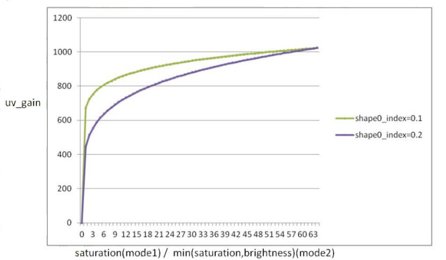

   

   Figure 3.17‑3 EE CA-Shape0 Function Illustration

2. shape1: S-shape

   It is recommended that the inflection point be fixed to zero, as shown by the purple line. shape1_index determines the curvature degree. The closer to 1, the greater the curvature degree, and the higher the suppression strength saturation.

   It is recommended to fix the inflection point at zero, as shown by the purple line. shape1_index determines the degree of curve bending; the closer it is to 1, the greater the curvature and the higher the saturation of suppression strength.

   

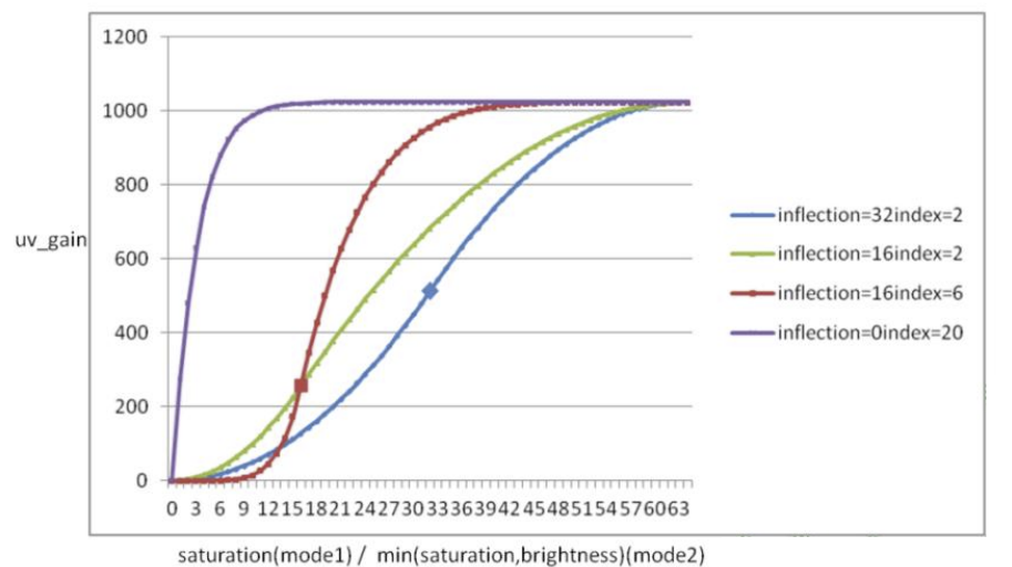
   Figure 3.17‑4 EE CA-Shape1 Function Diagram

3. shape2: parabolic shape

   Shape2_a determines the opening size of the parabola. The larger the Shape2_a, the smaller the opening, and the more saturated the suppression strength becomes.

   

   Figure 3.17‑5 EE CA-Shape2 Function Diagram

4. shape3: active shape

Five anchor points are activated to automatically generate the curve. Typically, the first anchor point is set at (0,0), and the fifth anchor point is set at (64,1024).

Figure 3.17‑6 EE CA-Shape3 Function Diagram

DCI

DCI is used to automatically generate curves based on predefined curves or histograms to improve global image contrast. The DCI curve consists of 64 points and can be manually adjusted using tools. Alternatively, it can be generated externally, with the dci_curve values copied into the JSON document.

Parameter	Type	Range	Description	Default Value
dciEnable	bool	{false,true}	true: enables the DCI curve. false: disables the DCI curve. This parameter is valid only if the value of curveEnable is 1.	false
dciCurve[65]	int[65]	[0, 1024]	The dynamic contrast improvement curve.	[0, 16, 32, 48, 64, 80, 96, 112, 128, 144, 160, 176, 192, 208, 224, 240, 256, 272,288, 304, 320, 336, 352, 368, 384, 400, 416, 432, 448, 464, 480, 496, 512, 528, 544, 560, 576, 592, 608, 624, 640, 656, 672,688, 704, 720, 736, 752, 768, 784, 800, 816, 832, 848, 864, 880, 896, 912, 928, 944, 960, 976, 992, 1008, 1023]

Table 3.17‑7 EE DCI Tuning Parameters

Color Processing

Overview

Color processing is performed by adjusting luminance and chrominance values, and can be configured to generate pixel values according to the ITU‑R BT.601 standard or full-range values. The input pixel range is also configurable, as YCbCr path pixels from the ISP may have two ranges depending on the camera sensor used.

Tuning Theory

Color-related terms are calculated as follows:

Contrast: Achieved by multiplying luminance values with the contrast value defined in the register.

Brightness: Adjusted by modifying the adjustment value defined in the register.

Saturation: Adjusted by multiplying Cr and Cb values with the fixed-point number defined in the register.

Hue: Phase shift of chrominance values.

More detailed explanations of how brightness, contrast, saturation, and hue adjustments are calculated are provided in the parameter descriptions.

Table 3.18-1 lists the parameters used in the color processing module.

Parameter	Type	Range	Description	Default Value
enable	bool	{true,false}	Enable/disable the CPROC module	true
contrast	float	[0,1992]	Y’=Y*(contrast), all pixels will be larger when contrast > 1	1
bright	float	[-127,127]	Real Bright= bright-64*(contrast-1)	0
saturation	float	[0,1.992]	UV’= 128 + (UV-128)*(saturation)	1
hue	float	[-90,90]	Rotation in HSV domain	0
chromaOut	int	[1,2]	Different RGB->YUV conversion matrix 1: limited range [16, 240] 2: full range [0, 255]	2

Table 3.18‑1 CPROC Tuning Parameters (8-bit)

Tuning during phase three

As a post-processing module, CPROC generally does not require special tuning in the first two stages of debugging and should remain at default values. In practical applications, contrast, brightness, saturation, and hue in the CPROC module can be dynamically adjusted based on different Gain values.

Color Noise Reduction (CNR)

Overview

Color noise typically manifests as random color shifts, color speckles, or uneven color distribution in digital images. These phenomena are mainly caused by uncertainties and noise during image acquisition or processing. To address this issue, the Chroma Noise Reduction (CNR) module in the Image Signal Processor (ISP)’s YUV domain is used to remove color noise.

The basic tuning procedure is as follows:

• Phase one: No tuning preparation required;

• Phase two: CNR module tuning for a primary scene under laboratory conditions;

• Phase three: Fine-tuning of CNR parameters to adapt to various scenes. Mainly based on gain to tune the corresponding modules;

Tuning Theory

The three-layer pyramid model used in chroma noise reduction is a multi-scale technique that allows image processing at different resolution levels, effectively removing noise while preserving important image details. In this model, Gaussian pyramids are a common method for constructing such a pyramid structure. The specific steps are as follows:

Bottom layer: The original image is directly used as the bottom layer of the pyramid.

Middle layer: Generated by applying Gaussian blur and downsampling to the bottom layer image. This step reduces image resolution while smoothing color variations, helping to remove noise.

Top layer: Further Gaussian blur and downsampling applied to the middle layer, resulting in a lower-resolution image layer.

At each layer, chroma noise reduction can be performed independently, then the processed layers are recombined to restore the original resolution. This method allows the algorithm to capture and remove noise at different scales while preserving image structure and details. In this way, the chroma noise reduction algorithm can more precisely control the denoising process, avoiding detail loss due to over-smoothing.

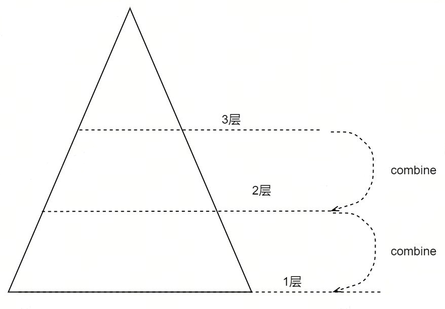
Figure 3.19‑1 CNR Processing Flowchart

The following are parameters related to CNR tuning.

Parameter	Type	Range	Description	Default Value
cnrEnable	bool	{true,false}	true: enables the chroma noise reduction (CNR) function. false: disables the CNR function.	false
cnrStrength	int	[0,128]	The denoise strength, which determines the degree to which the denoising result is merged back to the input image. If this parameter is set to 128, it indicates that 100% denoising result is used.	128
textureMaskSelect	int	[0,8]	Texture filter coefficient selection. The smaller the noise, the larger the parameter value should be set.	0
cSigmaLayer	float[3]	[1,96]	The sigma for each layer. The greater the noise intensity of a layer, the larger the parameter value should be set.	[16,16,12]

Table 3.19‑1 CNR Tuning Parameters

Tuning CNR during phase two

No other modules need to be tuned for CNR in phase one, but prior to phase two tuning, the following prerequisite modules must be tuned:

Prerequisite	Status/Value
Black level	Tuned
CCM	Tuned
DPC	Tuned
2DNR	Tuned
3DNR	Tuned
Demosaic	Tuned
Green Equalization	Tuned
Set Enable	0(disables CNR)

Table 3.19‑2 CNR Phase Two Prerequisites

To build the CNR tuning environment, illumination should be relatively low (e.g., 10 lux). The target can be a color chart inside a light box or a real scene, with rich color areas and gray patches in the scene to facilitate real-time assessment of color noise. The image appearance before CNR tuning is shown in Figure 3.19-2.

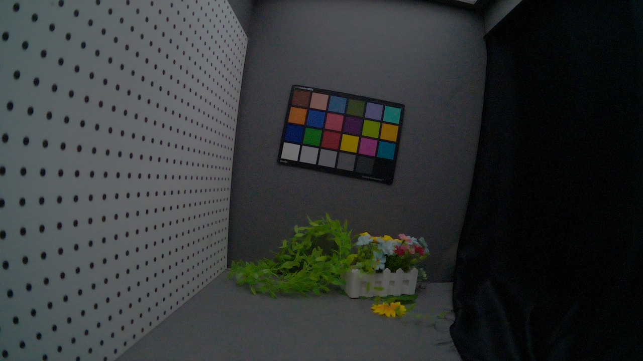
Figure 3.19‑2 Image Before CNR Tuning

Adjust the parameters related to the three-layer pyramid according to actual usage requirements to control the strength of CNR. Generally, start with default parameters and observe if the image appears normal. If color noise remains obvious, increase the cSigmaLayer value until the color noise meets requirements. If no obvious color noise is present, appropriately reduce cnrStrength and cSigmaLayer, or increase textureMaskSelect to weaken CNR’s impact on color reproduction. During tuning, avoid pursuing excessively strong noise reduction, as high denoising strength may introduce red/blue color cast risks. Figure 3.19-3 shows a reference example after tuning; actual noise levels after tuning should be adjusted based on usage requirements.

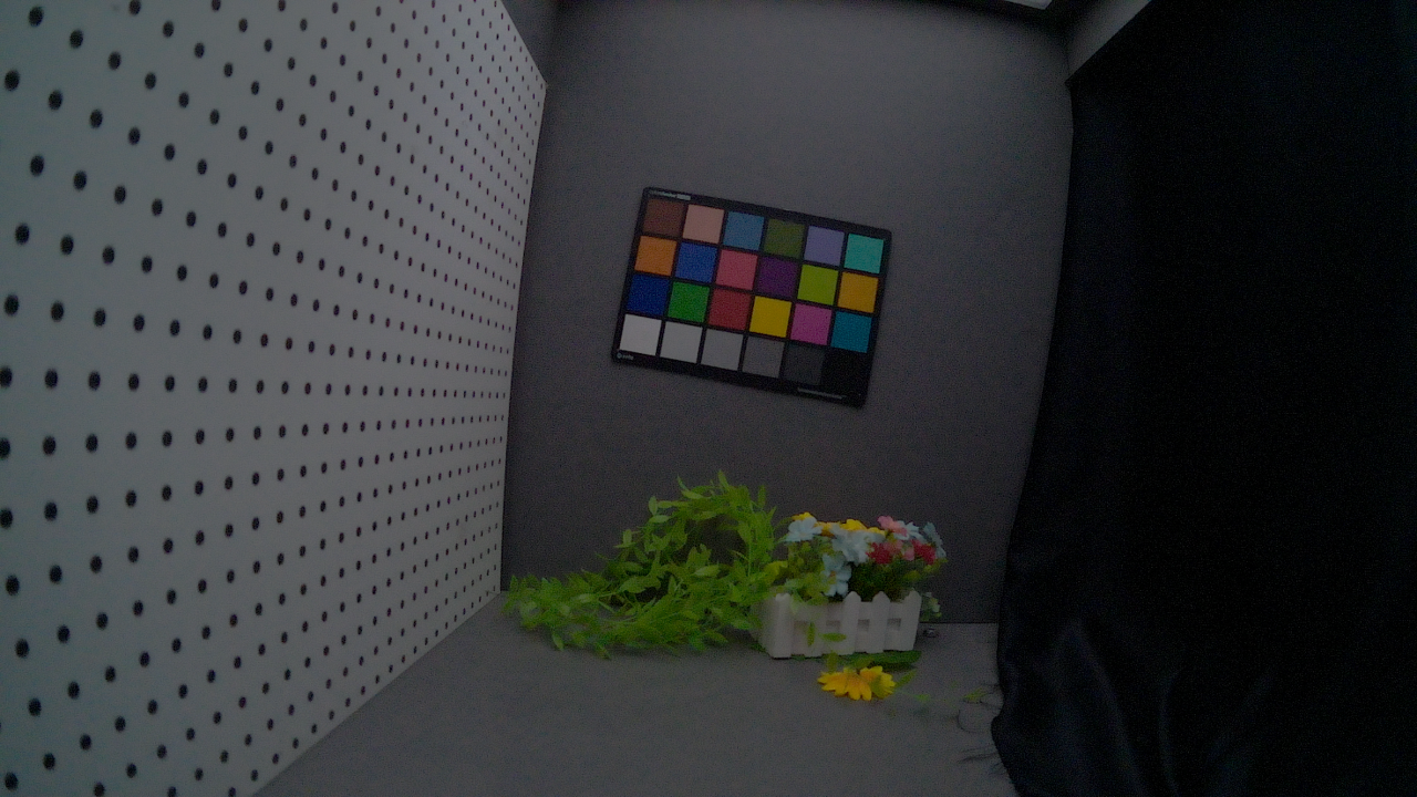
Figure 3.19‑3 Image After CNR Tuning

Fine Tuning CNR Phase Three

Change the lighting environment to obtain different gain values, repeat the phase two tuning process, and tune appropriate parameter values at each gain level. Once parameter tuning across the entire gain range is completed, CNR tuning is finished.

Auto Focus (AF)

Overview

Auto focus functionality should be determined based on usage scenarios regarding tuning frequency. For example, security cameras typically use manual focus, so auto focus is not required in such scenarios. In applications requiring auto focus, AF tuning is usually completed early in phase two. However, since AF module tuning is relatively independent, it can also be performed at other times. The specific AF tuning process is as follows:

• Phase one: No AF module tuning required, but manual focus adjustment is needed to meet imaging requirements. During this phase, the lens driver must be activated and tested to satisfy basic imaging functions.

• Phase two: Tune AF functionality to adapt to different scenes.

• Phase three: Before tuning AF, verify motor precision, speed, repeatability, and stability.

Tuning Theory

Auto Focus is a commonly used focusing technique whose basic principle is to achieve focus by comparing image sharpness.

In image processing, sharpness is usually measured by image contrast and high-frequency components. To achieve the clearest image, Auto Focus continuously adjusts image contrast and high-frequency components by changing the focal length.

The Auto Focus implementation process includes three steps: detecting sharpness, determining focus position, and moving the focus position.

In the first step, Auto Focus detects image sharpness using image processing algorithms.

In the second step, Auto Focus determines the current focus position based on sharpness detection results.

In the third step, Auto Focus moves the focus position according to the current focus position until the clearest image effect is achieved.

Repeat the above three steps until the image reaches maximum clarity.

The AF module supports two different auto focus technologies: CDAF and PDAF. The overall flowchart is as follows:

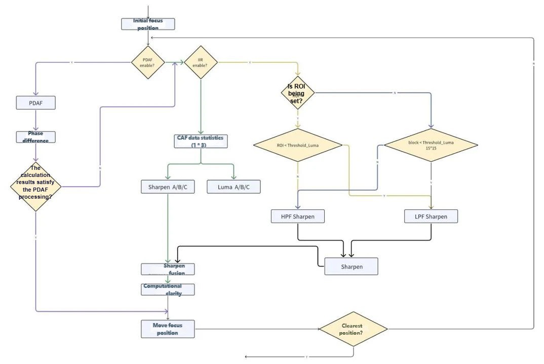
Figure 3.20‑1 AF Hybrid Focus Processing Flow

Function Description

CDAF (Contrast Detection Auto Focus) is an auto focus technology suitable for static shooting scenarios. It determines the focal point by comparing contrast in different image regions. The motor is moved within the minimum and maximum focal distance range to form a parabola of sharpness versus focal length. By locating the vertex of this parabola, CDAF finds the optimal focal length and maximum sharpness. Advantages of CDAF include high accuracy, suitable for high-resolution images, but disadvantages include insufficient speed for tracking moving objects.

PDAF (Phase Difference Detection Auto Focus) is an auto focus technology suitable for shooting moving objects. It uses phase difference information from the lens to determine the focal point. Defocus strength is detected via phase difference and converted into motor focal length using a defocus conversion coefficient. Advantages of PDAF include fast tracking speed for moving objects, suitable for high-speed motion scenarios, but disadvantages include relatively lower accuracy and potential for errors.

The software implementation flowchart of PD Split and PD Calibration in X5’s PDAF is shown below, supporting type2 mode.

type2: The sensor internally splits the PD information before outputting it to the backend for processing.

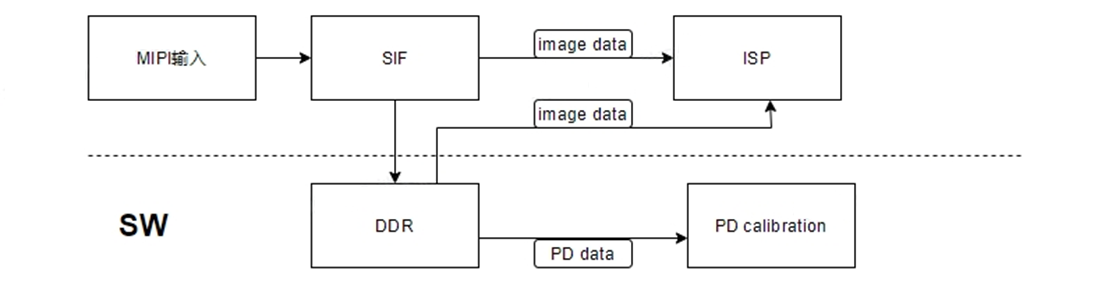
Figure 3.20‑2 PDAF Software Implementation Flow

AF Statistics

The AF statistics module (ISP_AFM) supports AF control. Most AF control tasks are completed in software. A search algorithm is used to find maximum sharpness in the image, and software controls lens movement based on statistical output of sharpness values. The hardware-implemented AF module provides image sharpness measurements via register interface.

Parameter	Type	Range	Description	Default Value
enable	bool	{true, false}	Whether to enable AF	true
maxFocal	uint16_t	[0,1023]	The maximum focal distance that the motor can reach.	600
minFocal	uint16_t	[0,1023]	The minimum focal distance that the motor can reach.	300

Table 3.20‑1 AF Basic Tuning Parameters

AF Control and Window Selection - CDAF

The AF module in hardware controls lens movement based on software commands. Software can select specific windows or regions of interest (ROI) in the image for focus measurement. This window selection helps focus on specific objects or areas within the image.

Window size is configured via registers, supporting up to 3 ROI regions by default in 3 columns. ROI positions can be adjusted by modifying (LT/RB) coordinates of each ROI, and each ROI’s weight is controlled by software.

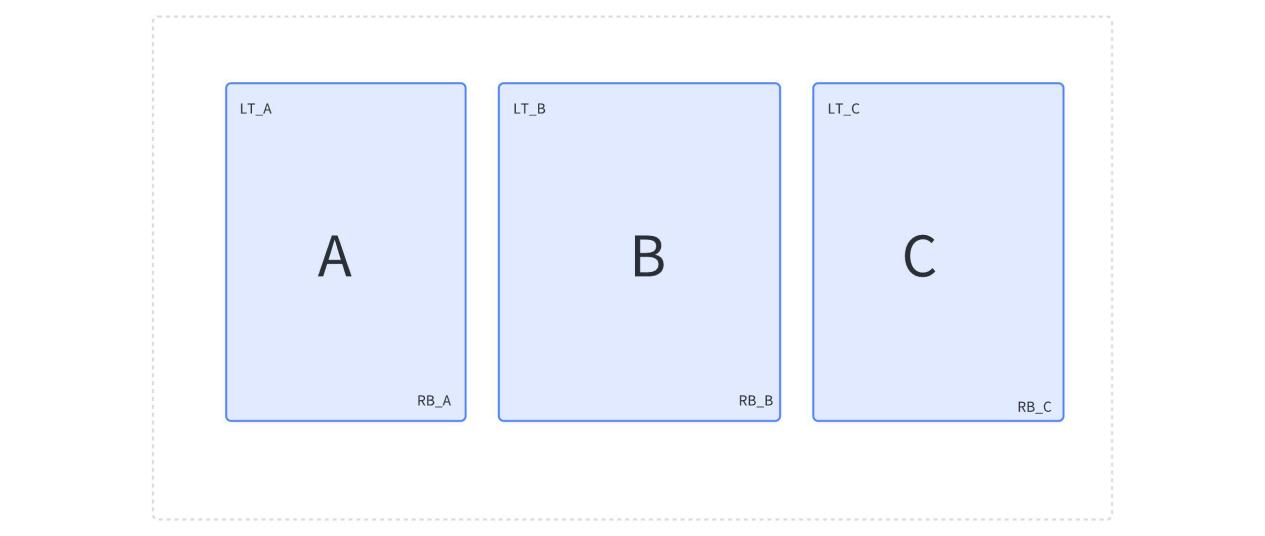
Figure 3.20‑3 CDAF ROI Region Configuration

AF Control and Window Selection - PDAF

Up to 48 windows can be configured. The specified ROI area is evenly divided into 48 windows, and each window’s weight is configurable.

The software internally supports Auto and Manual modes. In Auto mode, it defaults to a 3x3 window split with default weights. In Manual mode, users can customize the number and weights of windows.

IIR/FIR

IIR/FIR filter design flowchart in AF

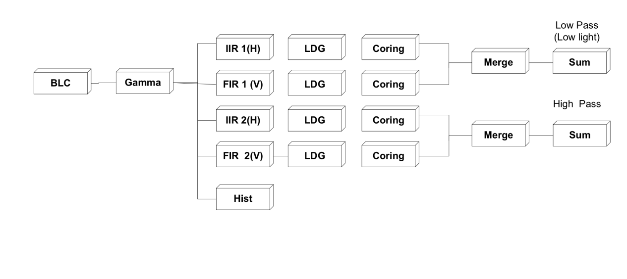
Figure 3.20‑4 IIR AF Processing Flow

The IIR filter divides the ROI region into a 15x15 grid. The offset position of the ROI can be adjusted by configuring blk_xpos and blk_ypos. blk_width and blk_height are used to set the size of each block.

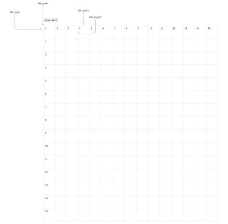
Figure 3.20‑5 IIR AF ROI Window Configuration

AF Statistical Sharpness Calculation

The auto focus module (AFM) can be programmed via configuration registers in the control register unit. Configuration changes are not allowed when AFM is enabled, as this may lead to unpredictable results.

The hardware statistics submodule of AF divides the image into multiple ROIs. For hardware statistics submodule V1, the number of ROIs is 9; for submodule V3, the number is 225.

For each ROI, sharpness is calculated using FIR and IIR filtering, with weights specified by weightWindow (for submodule V1) and afmV3WeightWindow (for submodule V3). The overall image sharpness is the weighted sum of sharpness from each ROI. Priority can be given to focusing on certain ROI areas by modifying the weights in the weightWindow[9] and afmV3WeightWindow[225] arrays.

Parameter	Type	Range	Description	Default Value
wightWindow	float[9]	[0,255]	ROI weight array for hardware statistics submodule V1.	1 for all elements
afmV3WeightWindow	float32_t[255]	[0,255]	ROI weight array for hardware statistics submodule V3.	1 for all elements

Table 3.20‑2 ROI Parameters

AF Mode Introduction

As previously mentioned, AF includes two auto focus modes: PDAF and CDAF. The actual modes available for focus adjustment are as follows:

• PDAF mode: Uses only PDAF. The focusing process includes initialization, search, lock, and wait.

• CDAF mode: Uses only CDAF. The focusing process includes initialization, search, tracking, lock, and wait.

• Hybrid mode: Uses both PDAF and CDAF. The focusing process initially undergoes PDAF initialization and search, followed by CDAF search, tracking, lock, and wait.

Mode selection can be made using the parameters in Table 3.20‑3.

Parameter	Type	Range/Description	Default Value
mode	enum	Selects the auto focus mode. The value range is: l (Default) CAMDEV_CDAF_INDIVIDUAL_MODE: CDAF mode. l CAMDEV_PDAF_INDIVIDUAL_MODE: PDAF mode. l CAMDEV_PDAF_CDAF_HYBRID_MODE: hybrid mode.	CAMDEV_CDAF_INDIVIDUAL_MODE

Table 3.20‑3 AF Mode Selection Parameters

PDAF Parameters Introduction

PDAF Statistical Calculation

PDAF search requires phase differences from ROIs. ROIs can be user-defined or default ROIs found by PDAF statistical calculation.

If using default ROI, the block with the smallest phase difference among all image blocks will be found and used as the ROI. If using user-defined ROI, a block can be selected as ROI using the pdRoiIndex parameter.

Parameter	Type	Range	Description	Default Value
pdRoiIndex	uint8_t	[0,48]	The selected ROI regions for PDAF focusing.	0

Table 3.20‑4 PDAF Statistical Calculation Parameters

PDAF Focusing

PDAF focusing can only proceed when PDAF confidence exceeds the threshold set by cPdConfThreshold.

A higher threshold imposes stricter confidence requirements on the image, making it harder to enter the PDAF focusing process. However, too low a threshold may cause focusing errors due to unreliable phase detection offset calculations.

Parameter	Type	Range	Description	Default Value
cPdConfThreshold	float	[0,1023]	PDAF confidence threshold.	300

Table 3.20‑5 PDAF Focusing Calculation Parameters

PDAF Searching

If the absolute value of phase difference remains below pdShiftThreshold for a consecutive number of frames (indicated by pdStableCountMax), the motor movement distance calculated by PDAF is considered correct. Then, if AF is in PDAF mode, PDAF locks; if AF is in hybrid mode, it proceeds to CDAF search.

Parameter	Type	Range	Description	Default Value
pdShiftThreshold	float32_t	(0,1)	The threshold for the absolute value of phase difference. The greater the parameter value, the faster the PDAF searching. However, PDAF stability cannot be guaranteed.	0.1
pdStableCountMax	float32_t	[1,10]	The number of frames to determine whether the PDAF focusing is completed. The smaller the parameter value, the faster the PDAF searching. However, PDAF stability cannot be guaranteed.	2

Table 3.20‑6 PDAF Search Speed Parameters

CDAF Parameters Introduction

CDAF moves the motor within the minimum and maximum focal distance range, forming a parabola of sharpness versus focal length. By finding the vertex of this parabola, CDAF locates the optimal focal length and maximum sharpness. To control computation speed, CDAF hill-climbing algorithm parameters cPointsOfCurve can be adjusted. Larger values result in slower computation but more accurate optimal focus position. Smaller values mean larger steps and faster computation speed. However, due to larger steps, the motor may skip the optimal focus position, leading to inaccurate focusing.

Parameter	Type	Range	Description	Default Value
cPointsOfCurve	uint8_t	[3,20]	Number of steps for the CDAF hill climbing algorithm.	12

Table 3.20‑7 CDAF Hill-Climbing Speed Parameters

Hybrid Mode Introduction

In most cases, PDAF and CDAF are used together in hybrid mode. However, using the parameters in the table below, the following special cases may occur:

• Using only PDAF without CDAF: Whether to use CDAF after PDAF search and the speed of CDAF search can be configured by setting parameters accurateFocusEnable and accurateFocusStep. If CDAF is disabled, hybrid mode is identical to PDAF mode.

• Using only CDAF without PDAF: This occurs when PDAF confidence remains zero for several consecutive frames during PDAF search. In this case, PDAF search is considered failed, and the AF module skips PDAF and directly starts CDAF search. lossConfidenceFrameNum can be set to control the threshold for PDAF search failure.

Parameter	Type	Range	Description	Default Value
accurateFocusEnable	bool	{true,false}	Whether to enable CDAF search after the PDAF search in hybrid mode. If it is set to false, the focus searching will stop after the PDAF search completes.	false
accurateFocusStep	uint8_t	[1,20]	The number of steps CDAF searches each time if CDAF search is enabled in hybrid mode. The smaller the parameter value, the faster the CDAF search and the poorer the focusing result.	5
lossConfidenceFrameNum	uint8_t	[1,20]	The number of frames to wait after PDAF loses confidence in hybrid mode. The greater the parameter value, the less likely to skip the PDAF search in hybrid focus mode.	3

Table 3.20‑8 Parameters Used in Hybrid Mode

AF Tuning During Phase One

As mentioned earlier, AF functionality does not require tuning in phase one. Therefore, in VTuner, the model can be set to AF_manual mode. In AF manual mode, the lens position can be manually adjusted via the position slider or by entering specific values in FocusControl to obtain a clear image.

Figure 3.20‑6 Manual AF Diagram

AF Tuning During Phase Two

Begin basic AF functionality tuning with the camera placed horizontally, following these steps:

1. Place an ISO12233 resolution chart or SFR gradient chart under 1000 lux illumination to identify image sharpness. The distance between the camera and chart should be infinity (greater than 2 meters).

2. In VTuner, set AF_mode_id to AF_calibration. In this mode, the command window outputs lens position and image sharpening parameters, separated by commas, as shown below.

   

Figure 3.20‑7 Lens Position (left) and Sharpening Parameters (right)

1. Use a plotting tool to graph the relationship between lens position and sharpening parameters on the same coordinate system to obtain the corresponding relationship between lens position and sharpening effect at infinity.

   

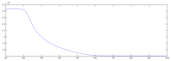
Figure 3.20‑8 Infinity Focus Response Curve

1. From the focus response curve, it can be seen that sharpness remains relatively stable before the 190LP position. The algorithm’s ideal point needs to detect a certain decrease in sharpness when the lens moves. Therefore, 190LP can be determined as the focus point under infinity conditions.

2. Repeat the above steps several times to confirm the accuracy of the LP value. Typically, a 1% deviation range is acceptable. If test results fall within this accuracy range, the lens position value can be entered into the corresponding AF_lms infinity field.

3. Reduce the obtained infinity lens position LP by 15% to obtain the lens position for far-end focusing, i.e., infinity LP × 0.85. Enter this value into the corresponding LUT location.

4. To obtain the focus position for macro conditions, use a small resolution chart under 1000 lux illumination, setting the distance between the camera and resolution chart to 10 cm. Run calibration mode to obtain the focus response curve.

   

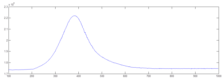
Figure 3.20‑9 Macro Focus Response Curve

1. From the above figure, obtain the LP corresponding to the highest sharpening point and enter this value into the AF_lms position corresponding to macro. Data shows maximum sharpening occurs at 384 LP; repeat several times to confirm focus accuracy.

2. The near-end focus point LP can be obtained by increasing the macro LP value by 10%, i.e., macro LP × 1.1. Enter this value into the calibration LUT.

   Repeat the above operations to obtain LP values for lens-up and lens-down orientations, and enter these values into the corresponding positions in the dynamic_calibration.c file, as shown in the table below.

| **Parameter** **name** | **Description**                                 |
| ---------------------- | ----------------------------------------------- |
| Down_FarEnd            | Downward orientation FarEnd lens position       |
| Horizontal_FarEnd      | Horizontal Orientation FarEnd lens  position    |
| Up_FarEnd              | Upward Orientation FarEnd lens position         |
| Down_Infinity          | Downward orientation Infinity lens  position    |
| Horizontal_Infinity    | Horizontal orientation inifinity lens  position |
| Up_Infinity            | Upward orientation inifinity lens position      |
| Down_Macro             | Downward orientation macro lens position        |
| Horizontal_Macro       | Horizontal orientation macro lens position      |
| Up_Macro               | Upward orientation macro lens position          |
| Down_NearEnd           | Downward orientation NearEnd lens position      |
| Horizontal_NearEnd     | Horizontal orientation NearEnd lens  position   |
| Up_NearEnd             | Upward orientation NearEnd lens  position       |

Table 3.20‑9 AF Basic Calibration Parameters

AF control operation calibration parameters are listed in the following table.

Parameter name	Description
Step_Number	The total steps from FarEnd to NearEnd
Skip_frames-in	Number of frames be skipped before AF start
Skip_frames_moves	Number of frames be skipped before each AF iteration
Dynamic_range_th	Focus Value Contrast threshold
Spot_tolerance	Focus value dynamic range minimum threshold of zones which used to filter out unqualified ROI in multi-spot
Exit_th	Focus Value downhill threshold
Caf_trigger_th	CAF scene change trigger threshold
Caf_stable_th	CAF scene change stable threshold

Table 3.20‑10 AF Extended Calibration Parameters

In the VTunerClient tool, Caf_trigger_th needs to be tuned to detect actual scene changes. When the change magnitude of actual scene characteristics exceeds the Caf_trigger_th threshold, CAF adjustment will be triggered. The Caf_stable_th parameter is used to judge scene stability; the change magnitude of actual scene characteristics should be less than the set value of Caf_stable_th. Once the scene characteristic value exceeds Caf_trigger_th or falls below Caf_stable_th, CAF adjustment will occur.

AF Tuning During Phase Three

After completing auto focus tuning in phase two, re-tuning is generally not required; AF functionality can already be used to focus on various scenes. In VTuner, specific AF_mode_id modes such as AF_auto_single or AF_auto_continuous can now be selected for use.

AF_auto_single - When manual focus is required for each new scene change, select AF_auto_single mode. The camera will focus on the current scene and stabilize the VCM at the final LP. To re-focus or switch to another scene, repeat the above operation.

AF_auto_continuous - When AF_auto_continuous mode is selected, the system continuously refreshes focus data to find the optimal focus position. In this mode, the system continuously provides optimal focus points for different scenes, meaning this mode requires stronger processing power compared to AF_auto_single.