4.1.1.7. Model Performance Analysis and Optimization

This section describes how to evaluate model performance using the tools provided by D-Robotics. If the evaluation results are not found to be as expected at this stage, it is strongly recommended that you try to resolve performance issues at this stage, based on D-Robotics’ optimization recommendations. It is not recommended to extend model problems into the application development phase.

4.1.1.7.1. Use the hb_perf Tool to Evaluate Model Performance

The hb_perf provided by D-Robotics takes the *.bin obtained from the model conversion as input and can directly obtain the expected on-board performance of the model. The tool is used as follows:

hb_perf  ***.bin

Note

If you are intended to analyze the packed model after running the pack command, you need to add a -p parameter and run hb_perf -p ***.bin. For the pack command, please refer to the Other Dev Tools (Optional) section.

The *.bin in the command is the bin model of the model conversion output. After the command is executed, a hb_perf_result directory will be generated in the current working directory, and the analysis results will be provided in html format. The following is a sample result of our analysis of a MobileNet, where mobilenetv1_224x224_nv12.html is the main page to view the analysis results

hb_perf_result/
└── mobilenetv1_224x224_nv12
    ├── MOBILENET_subgraph_0.html
    ├── MOBILENET_subgraph_0.json
    ├── mobilenetv1_224x224_nv12
    ├── mobilenetv1_224x224_nv12.html
    ├── mobilenetv1_224x224_nv12.png
    └── temp.hbm

Open the main page using your web browser, you’ll see the following:

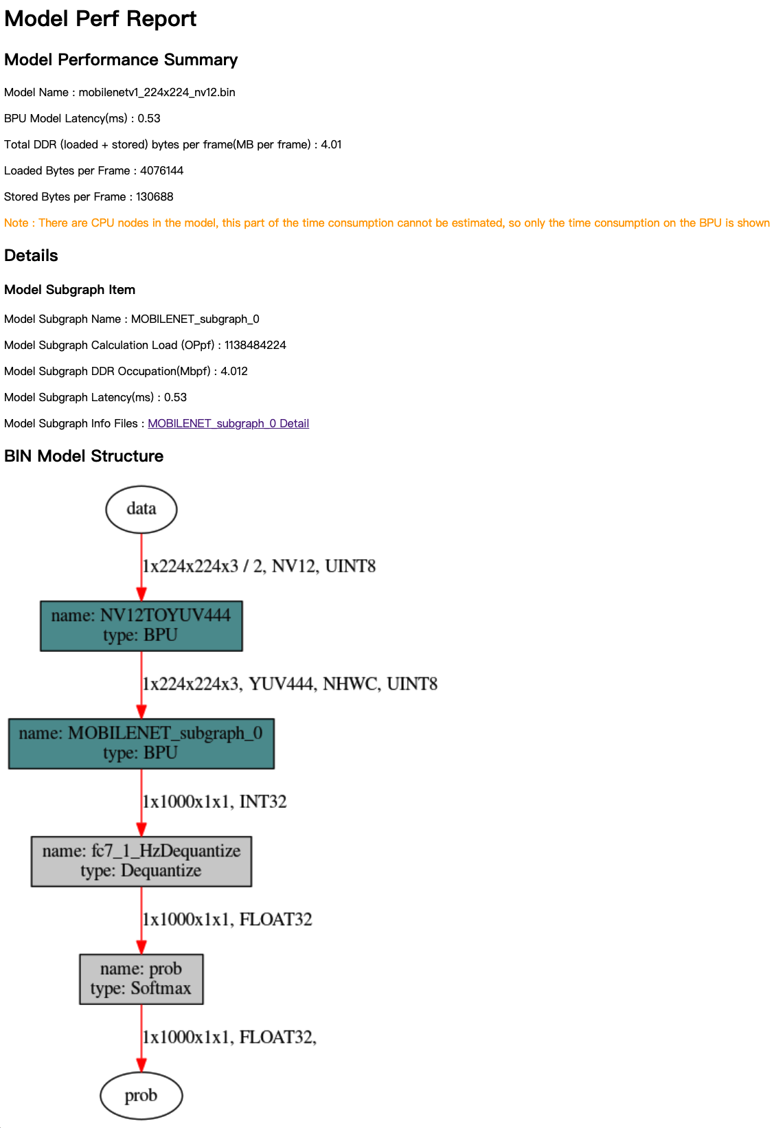
Analysis results consist of 3 parts: Model Performance Summary, Details and BIN Model Structure. Model Performance Summary is the overall performance evaluation result of the bin model. Wherein, the indicators represent respectively:

• Model Name——model name.

• Model Latency(ms)——model’s overall time consumption of single frame computing (in ms).

• Total DDR (loaded+stored) bytes per frame (MB per frame)——total amount of DDR used for data loading and storage in the overall BPU part of the model (in MB/frame).

• Loaded Bytes per Frame——model’s data loading volume per frame during execution.

• Stored Bytes per Frame——model’s data storing volume per frame during execution.

You need to understand the concept of subgraph before learning Details and BIN Model Structure. If there are CPU computing OPs in the non-input or output part of the model, the model conversion tool will split the OP’s continuous BPU computing part into 2 independent subgraphs. For details, please refer to the Check the Model section.

Details refers to the detailed information of each model’s BPU subgraph(s). The indicators of each subgraph in the main page are shown as below:

• Model Subgraph Name——name of the subgraph.

• Model Subgraph Calculation Load (OPpf)——single frame computing load of the subgraph.

• Model Subgraph DDR Occupation(Mbpf)——single frame loading/writing volume (in MB) of the subgraph.

• Model Subgraph Latency(ms)——single frame computing time consumption of a the subgraph (in ms).

Each subgraph provides a detailed page, in which you can get more specific information. All the above indicators are obtained from the detailed page.

Attention

Note that the detail page will differ depending on whether you have the debug parameter (debug) enabled or not. In below, the Layer Details can only be obtained when the debug parameter in the configuration file is specified as True. For the configuration of the debug parameter please refer to the Convert The Model Using The hb_mapper makertbin Tool section.

BIN Model Structure is a subgraph level visualization results of bin model, in which the nodes in dark color represent those subgraphs run on the BPU; while the nodes in gray represent those nodes computed in CPU.

Layer Details analyzes specific OP-level information, it is a useful reference in the debugging and analysis stage, especially when there is low model performance problem caused by BPU OPs, it can help you find the problematic OPs.

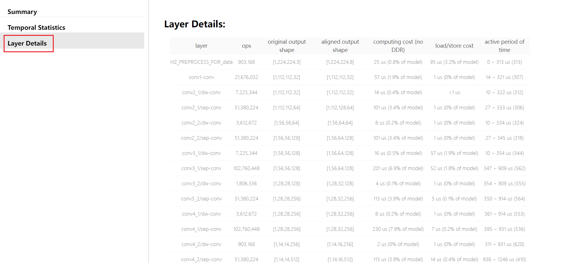
Of these, each indicator is explained below:

• layer: layer name.

• ops: computation amount.

• original output shape: output shape of original op.

• aligned output shape: output shape of aligned op.

• computing cost (no DDR): computation time.

• load/store cost: data handling time.

• active period of time: the active time period of the compiled layer (does not represent the execution time of the layer, usually multiple layers alternate/execute in parallel).

The purpose of using the hb_perf is to understand the subgraph structure of bin model. In addition, this tool can also provide comprehensive static analysis indicators. But the hb_perf doesn’t include the computing evaluation of the CPU part, however, this is not a big deal as long as CPU computations only cover those regular processing at the model input or output parts without those extensive computing nodes. Otherwise you’ll need to utilize some dev board tool to evaluate the actual model performance.

4.1.1.7.2. Evaluate Actual Model Performance on Dev Board

The hrt_model_exec perf tool is used to evaluate actual model performance on dev board. The hrt_model_exec is a model execution tool that can evaluate models’ inference performance and obtain model information. On the one hand, it enables users to get models’ actual performance, on the other hand, it helps users to learn the speed limit that the model can achieve, which is a guideline for the target limit of application optimization.

Before using hrt_model_exec perf tool, there are two preparations:

1. Make sure you have referred to the Environment Deployment to complete the installation of the tools on the development board.

2. Copy the bin models from your Ubuntu dev machine to the dev board (recommended to put it in the /userdata directory). As there is a Linux operating system on the dev board, you can use some popular Linux commands, such as the scp to copy the models.

Note

The model used at this time does not need to enable debug, debug enabled will affect the test results of the model on the development board.

The reference command for the actual performance test using hrt_model_exec perf is shown as follows (Note that it is executed on the development board):

./hrt_model_exec perf --model_file mobilenetv1_224x224_nv12.bin \
                      --model_name="" \
                      --core_id=0 \
                      --frame_count=200 \
                      --perf_time=0 \
                      --thread_num=1 \
                      --profile_path="."

Among them, the meaning of each parameter is shown as follows.

model_file: The name of the bin model.

model_name: This parameter requires the name of the BIN model to be analyzed. Note that the name can be omitted when only one model is specified by the model_file.

core_id: The default value is 0. This parameter specifies the core ID to run the model. 0 denotes arbitrary core; 1 denotes core 0; 2 denotes core 1. You can specify it as 0 when analyzing the limit of both cores.

frame_count: The default value is 200. This parameter specifies the inference frame number. The tool will execute the specified number of times, and then analyze the average time consumption. It will become valid when the perf_time is specified as 0.

perf_time: The default value is 0. Measured by minute. It denotes inference time, the tool will analyze the average time consumption when completing the specified execution time.

thread_num: The default value is 1. It is used to specify the number of thread and the value range is [1,8]. To analyze the limit frame rate, you need to increase the number of thread.

profile_path: By default it is off. It is used for specifying the path to generate log. Analysis results will be save into the profiler.log file and the profiler.csv file in specified path.

You will see the following message at the console after running this command. As shown below, the Average latency and Frame rate respectively denotes the average single frame inference latency and the limit frame rate of the model. If you want to get the speed limit of model on dev board, you will need to increase the thread_num till it is good enough.

Running condition:
  Thread number is: 1
  Frame count   is: 200
  Program run time: 818.985000 ms
Perf result:
  Frame totally latency is: 800.621155 ms
  Average    latency    is: 4.003106 ms
  Frame      rate       is: 244.204717 FPS

There are only overall messages shown at the console, you can control the profiler.log file and the profiler.csv file by specifing the profile_path parameter in order to generate more detailed information.

{
  "perf_result": {
    "FPS": 244.20471681410527,
    "average_latency": 4.003105640411377
  },
  "running_condition": {
    "core_id": 0,
    "frame_count": 200,
    "model_name": "mobilenetv1_224x224_nv12",
    "run_time": 818.985,
    "thread_num": 1
  }
}
***
{
  "processor_latency": {
    "BPU_inference_time_cost": {
      "avg_time": 3.42556,
      "max_time": 3.823,
      "min_time": 3.057
    },
    "CPU_inference_time_cost": {
      "avg_time": 0.29193,
      "max_time": 0.708,
      "min_time": 0.101
    }
  },
  "model_latency": {
    "BPU_MOBILENET_subgraph_0": {
      "avg_time": 3.42556,
      "max_time": 3.823,
      "min_time": 3.057
    },
    "Dequantize_fc7_1_HzDequantize": {
      "avg_time": 0.12307,
      "max_time": 0.274,
      "min_time": 0.044
    },
    "MOBILENET_subgraph_0_output_layout_convert": {
      "avg_time": 0.025945,
      "max_time": 0.069,
      "min_time": 0.012
    },
    "Preprocess": {
      "avg_time": 0.009245,
      "max_time": 0.027,
      "min_time": 0.003
    },
    "Softmax_prob": {
      "avg_time": 0.13366999999999998,
      "max_time": 0.338,
      "min_time": 0.042
    }
  },
  "task_latency": {
    "TaskPendingTime": {
      "avg_time": 0.04952,
      "max_time": 0.12,
      "min_time": 0.009
    },
    "TaskRunningTime": {
      "avg_time": 3.870965,
      "max_time": 4.48,
      "min_time": 3.219
    }
  }
}

The content here corresponds to the bin visualization diagram presented in the BIN Model Structure section of Use The hb_perf Tool To Evaluate Model Performance . Each node in the diagram has a corresponding node in the profiler.log file, which can be matched by name. The execution time of each node is recorded in the profiler.log file, which is an important reference for optimizing the nodes. Since the BPU nodes in the model have special requirements for input and output, such as special layout and padding alignment requirements, so the input and output data of the BPU nodes need to be processed.

• Preprocess: indicates the padding and layout conversion operation for the model input data, and its time consumption statistics are in Preprocess.

• xxxx_input_layout_convert: indicates the operation of padding and layout conversion for the input data of BPU nodes, and its time consumption statistics is in xxxx_input_layout_convert.

• xxxx_output_layout_convert: indicates the operation of removing padding and layout conversion from the output data of the BPU node, and its time consumption statistics is in xxxx_output_layout_convert.

The profiler analysis is a frequently used operation, The previous Interpret Model Check Results section mentioned that the check phase should not focus too much on CPU operators, at this stage, you can see the exact time consumption of the CPU operator. If the CPU time is considered too long based on the evaluation here, it is worth optimizing.

4.1.1.7.3. Model Performance Optimization

This section deals with the cases when you find out that the model performance in the above analysis results fails your expectations. It is composed by below subsections:

• Check Those Performance-affecting YAML Configuration Parameters;

• CPU OP Processing;

• High Performance Model Design Proposal;

• Use D-Robotics Platform Friendly Structure & Model.

Because some optimizations may influence the parameter space of the original floating-point model, in other words, it may cause model retraining. To prevent the costs of repeated adjustments and retraining brought about by model performance optimization, we suggest that you use random parameters to export models and validate performance before getting satisfactory model performance.

Check Those Performance-affecting YAML Configuration Parameters

Some parameters in the model conversion configuration file can affect model’s final performance, you can check if they’ve been correctly specified as you expected. The definitions and functions of all parameters please refer to the Specific Parameter Information section.

• The layer_out_dump parameter is used to specify whether to dump the intermediate results in model conversion. Strictly speaking, this is only a debugging parameter. It will add a dequantized output node to each convolutional operator and hence significantly reduce model’s onboard performance when specified as True. Therefore, please remember to specify it as False in performance evaluation.

• The compile_mode parameter is used to select whether the optimization direction is bandwidth or latency when compiling the model. If you are concerned about performance, please configure it as latency.

• The optimize_level parameter is recommended to be specified as O3 when you are going to deliver your product in order to obtain better onboard performance.

• The core_num : when the parameter is configured to 2, two cores can be called at the same time, reducing the inference latency of a single frame, but also affecting the overall throughput rate.

• The debug : If this parameter is set to True, the debug mode of the compiler will be turned on, which can output performance simulation related information, such as frame rate, DDR bandwidth usage, etc. This parameter is generally used in the performance evaluation stage. It can be turned off to reduce the model size and improve the model execution efficiency.

• The max_time_per_fc parameter is used to control the execution time of the function-call of the compiled model data instruction, thus implementing the model priority preemption function. Setting this parameter to change the execution time of the function-call of the preempted model will affect the on-board performance of the model.

CPU OP Processing

When it is confirmed by the hrt_model_exec perf’s evaluations that the performance bottleneck lies in CPU OPs, we suggest that you should confirm if the OPs which currently running on the CPU can be supported by the BPU as described in the Model Conversion Toolchain Operator Support Constraint List section.

If the OP(s) can be supported by the BPU, then it must be the case that your OP parameters have exceeded the BPU supported parameter restrictions. In such case, just adjust the corresponding computing parameters of the original floating-point model back into the restricted range. To help you quickly find out the off-limits parameter(s), we suggest that you proceed the model check procedure as described in the Check the Model section, the tool will print out the off-limits parameters at the console.

Note

Note that you’ll need to handle the effect on model performance (if any) caused by modifying the original Floating-point model parameters. Take the input_channel or output_channel of Convolution exceeding restrictions as classic examples, by reducing number of channels to quickly enable the OP to be supported by the BPU can also affect model accuracy.

If the operator does not have BPU support, you need to optimize it according to the following conditions:

• CPU operator at the middle of the model

  For cases where the CPU operator is in the middle of the model, it is recommended that you try parameter adjustment, operator replacement or model modification as a priority.

• CPU operator at the beginning and end of the model

  For the case where the CPU operator is at the beginning and end of the model, please refer to the following example, using the quantization/anti-quantization nodes as an example.

  • For nodes connected to the model input and output, you can add the remove_node_type parameter to the yaml file model_parameters configuration group (model parameters group) and recompile the model.

    remove_node_type: "Quantize; Dequantize"
    

    Or use the hb_model_modifier tool to make changes to the bin model:

    hb_model_modifier x.bin -a Quantize -a Dequantize
    

  • For models like the one below that are not connected to input and output nodes, you need to use the hb_model_modifier tool to determine whether the connected nodes support deletion, and then delete them one by one in order.

    

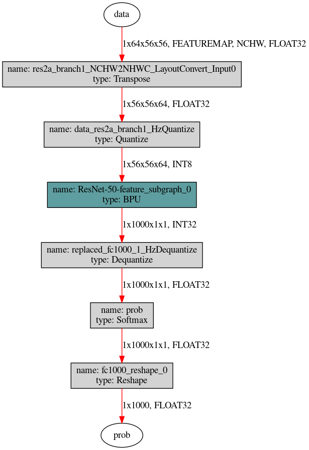
    Firstly, use the hb_perf tool to get the model structure picture, and then use the following two commands to remove Quantize nodes from top to bottom. The Dequantize nodes can be deleted one by one from bottom to top, and the names of the nodes that can be deleted at each step can be viewed by hb_model_modifier x.bin.

    hb_model_modifier x.bin -r res2a_branch1_NCHW2NHWC_LayoutConvert_Input0
    hb_model_modifier x_modified.bin -r data_res2a_branch1_HzQuantize
    

High Performance Model Design Proposal

Based on the performance evaluation results, you can see that the CPU time consumption proportion is actually very small and that the major performance bottleneck lies in the prolonged BPU inference time consumption. In such cases, as we’ve already utilized all computing components, the remaining optimization space lies in the use ratio improvement of computing resources. Since each processor has its own hardware characteristics, whether the computing parameters of algorithm models fit hardware characteristics well can directly determine the use ratio of computing resources. The better they fit, the higher the utilization rate, and vice versa. This section elaborates the hardware characteristics of D-Robotics’ hardwares.

Firstly, D-Robotics’ computing platform are designed for CNN (Convolution Neural Network) acceleration and the major computing resources are made for processing all types of convolutions. Therefore, your models are expected to be convolution-oriented, any other types of OPs can lead to reduced computing resource utilization and the impact varies depending on different OPs.

Overall Hardware Requirements

Below table lists some hardware level computing-friendly requirements for your reference.

OPERATOR	RESTRICTION	NOTE
Convolution	Kernel HxW=[1,7]x[1,7]	It can cause waste of computing power when the kernel size equals 2, 4 or 6
	Channel Num (one group) <= 2048
	Conv with sumin: Stride∈{1, 2}, Others: no restriction	It can cause waste of computing power when the Stride > 2. It can lead to additional padding operations when the Pad doesn’t equal kernel_size/2 and hence cause reduced model performance.
	Dilation value must be divisible by stride	Dilation can lead to additional data migration.
	Size of Kernel: HxWxC <= 32768
Deconvolution	Kernel HxW=[2,14]x[2,14]	Deconvolution is not natively supported by BPU.
	Channel Num <= 2048
	Padding HxW=[0,(Kernel_H-1)/2]x[0,(Kernel_W-1)/2]
	Stride ∈ {2, 4}
Fully Connected Convolution	Kernel HxW=[1,31]x[1,31], and HxW <= 127
	Channel Num∈[1,2048], or <= 16384 if H and W are both 1
	for int8 output: HxCEIL(W/8)xCEIL(C/4) <= {512(X2/J2), 1024(X3)}
	for int32 output: HxCEIL(W/8)xCEIL(C/4) < {1024(X2/J2), 2048(X3)}
Pooling	Average pooling: Kernel HxW=[1,7]x[1,7], Stride∈{1, 2}, Padding HxW=[0,Kernel_H/2]x[0,Kernel_W/2]
	Global average pooling: Kernel HxW <= 8192
	Max pooling: Kernel HxW=[1, 64]x[1,64], Stride=[1,256], Padding >= 0	There can be additional costs when Padding > 1 and Stride > 2.
	Global max pooling: Kernel HxW=[1,1024]x[1,1024]
Upscale	Scaling proportional range (1/256,256], precision=1/256
RoiAlign/Roiresize	Scaling proportional range (1/256,256], precision=1/256
Channel Concat	None	Time consumption will increase when the channel num of the Input feature is not multiples of 4.
Channel Split	Input feature channel is multiple of split number.	Time consumption will increase when the channel num of the Output features is not multiples of 4.
Slice	None	Time consumption will increase when the W in the starting coordinates is not multiples of 8. The slice alongside channel direction can occupy MAC computing resources.
Upsample	mode={nearest}, HxWxC -> (2H)x(2W)xC
Reshape	Reshape in the H and W directions, currently N and C are not supported.	Time consumption can be mass when the W of the Input/Output feature is not multiples of 8.
	reorder upscale: HxWxC -> (2H)x(2W)x(C/4)
	stack neighbor: HxWxC -> (H/2)x(W/2)x(4C)
Shuffle	Input feature channel <= 2048, only supports shuffle in C direction	It can occupy MAC computing resources if the granularity of shuffle is not multiples of 4.
Elementwise Add	Input feature channel <= 2048	It can occupy MAC computing resources.
Elementwise Mul	Input feature channel <= 2048	It can occupy MAC computing resources and has lower efficiency.
Broadcast Mul	Input feature channel <= 2048	It can occupy MAC computing resources and has lower efficiency.
Elementwise Max/Min	Input feature channel <= 2048	It can occupy MAC computing resources and has lower efficiency.
LookupTable (sigmoid,tanh..)	Lookup table: int8 -> int8	It can occupy MAC computing resources and has lower efficiency.
Pad	Pad Zero, Constant or Boundary
Cross Channel Max	Input feature channel ∈ [1, 64*group_num].
Detection Post Process	Filter + Sort + NMS
	Anchor num: [1, 64], Class num: [1, 64]
	Max output num: 4096
Leaky Relu	None	It can occupy MAC computing resources and has lower efficiency.
Prelu	None	It can occupy MAC computing resources and has lower efficiency.
Relu/Relu6	None	It can occupy MAC computing resources and has lower efficiency.

Convolution Width Alignment

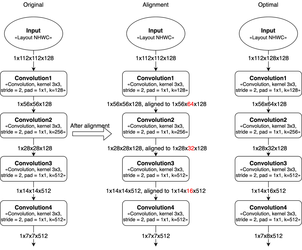
Due to the alignment requirement when computing MAC array, it can increase the efficiency when W of featuremap is multiples of 8 (when Convolution stride = 2, W should be multiples of 16). There can cause waste of computing power and lead to reduced MAC utilization when the above-mentioned W alignments don’t satisfy the multiples of 8 or 16 requirements. For example, when the input feature size of convolution is 1x8x9x32 (NHWC), in actual computations, the W will be padded as 15 (i.e. the feature size becomes 1x8x16x32) and will cause waste of computing resources.

When designing the network, the MAC utilization will be directly increased if the input size (align upwards or downwards) of the entire neural network can be changed.

Below is an sample in which displays the differences of model input sizes equal 224 or 256/192 when there is a multi-layered network (based on ResNet) whose stride=2.

Convolution Channel Alignment

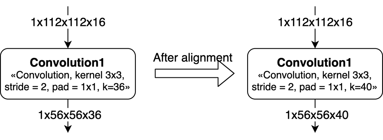
As the Channel must be multiples of 8 in hardware, it is better to adjust the kernel num to multiples of 8 when designing the algorithm.

The alignment of the channel of Group Convolution is more complicated.

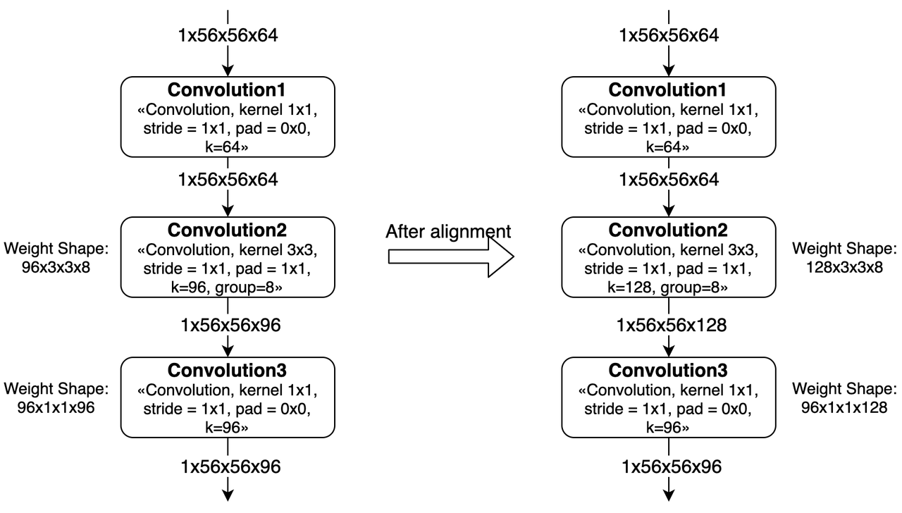
If the Kernel doesn’t equal integer multiples of 8, then the kernel num of each group need to be multiples of 8. Also, the alignment here can cause waste of computing power in subsequent convolution. As shown in the above frame digram, after padding the weight in Convolution2, the other weight in the next layer will also require padding.

Note

The padding method is to align each group with multiples of 8, i.e., padding data spread over weight.

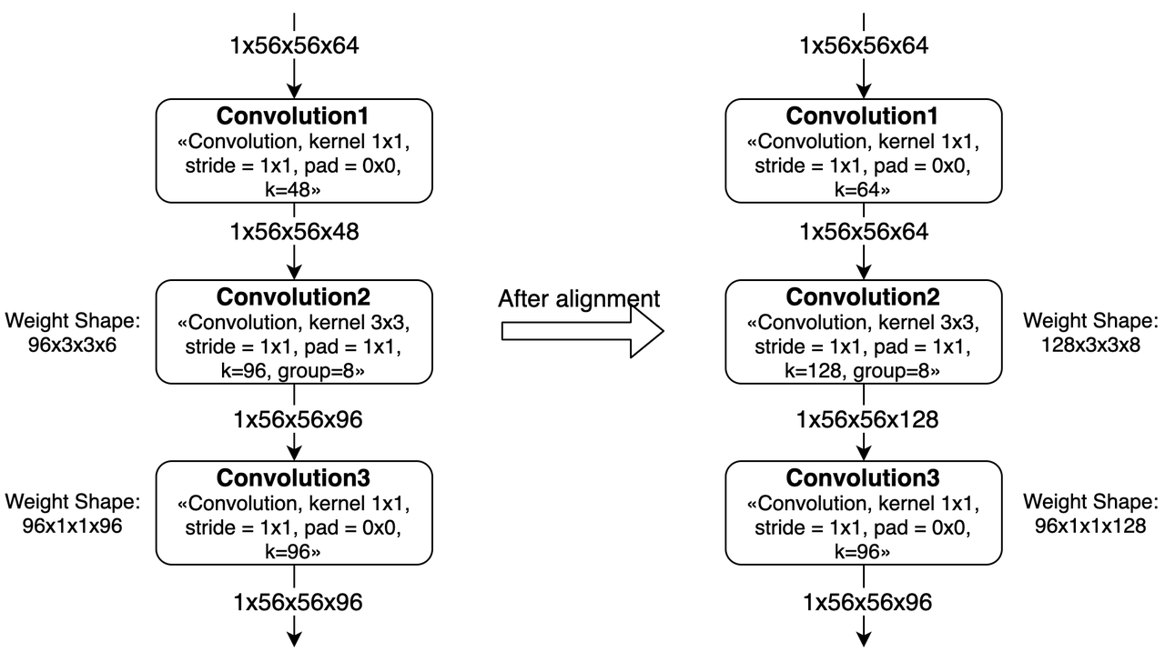
If the channels in group is not multiples of 8, then the convolutions of the upper layer must proceed padding. As shown in the above frame diagram, Convolution1’s kernel num is modified from 48 into 64 by padding.

In addition, there can be greater impact when multiple consecutive unaligned kernel number or channel number take place in the groups of group convolution. In such cases, we’ll need to consider the alignment requirements of multi-layer group conv at the same time and can cause more padding. At worst, the group convolution will be converted into ordinary convolution.

Activation Function

Most activation functions require to use LUT and Element-wise OP implementations, although LUT and element-wise operations can be supported now, they are all combinations of other OPs whose efficiency are too high.

In case there are only a few places in the model where you need to use some activation functions (non-relu) who are not supported by the hardware but have less computation costs, they won’t affect the computing efficiency of the entire model on a large scale.

However, when there are a large volume of activation functions who are not supported by the hardware in the model, they can have great impacts on the model’s execution speed.

Other Suggestions

The computational efficiency of depthwise convolution on the horizon computing platform is close to 100%, the BPU has an efficiency advantage on the MobileNet models.

In addition, when designing the models, the time consumption and hardware’s bandwidth pressure caused by those quantization and dequantization nodes can be relieved by reducing the input/output dimensions at the models’ BPU segments. Taking the classic segmentation models as an example, we can directly merge the Argmax operator into the model. Note that the Argmax operator can support BPU acceleration only when the following conditions are met:

1. By default, the axis of the Softmax layer in Caffe equals 1, however the the axis of ArgMax layer equals 0 by default, so please keep the axis value the same when replacing the operator.

2. The Channel of Argmax should be ≤ 64, otherwise it can only be computed on the CPU.

BPU High-efficiency Model Optimization

The academic community is continuously optimizing the computational efficiency (the smaller the theoretical computation required for the same algorithm accuracy, the higher the efficiency) and parameter efficiency (with the same algorithm accuracy, the less the parameter volume, the higher the efficiency) of algorithm models. The representative operations, such as the EfficientNet and the ResNext, have utilized the Depthwise Convolution and the Group Convolution respectively. However, as the supporting efficiencies of GPU and TPU are very low and cannot make full use of algorithms’ advantages when confronting such high-efficient models, hence the academic circle was forced to optimize the EfficientNetV2 and the NFNet for GPU/TPU. The optimizations primarily lie in less use of Depthwise Convolution and significantly expanding the Group size in Group Convolution. As a results, these modifications have reduced the computation and parameter efficiencies of the original models.

D-Robotics’ X3-BPU and J3-BPU have made specific optimizations for Depthwise Convolution and Group Convolution, making it possible for users to obtain higher computation and parameter efficiencies.

As reference samples of the 2 models, Algorithm Toolchain’s model_zoo release package proudly provides:

• The efficientnet[-lite] series with a quest for superb computation and parameter efficiencies. The X3-BPU can provide efficiently support: take the EfficientNet Lite0 as example, the X3-BPU’s frame rate is 6x higher than some 30TOPS GPU.

• The VarGNet series, D-Robotics’ own-developed models who take full advantages of Group Convolution’s high efficiency and optimized the X3-BPU and J3-BPU at the same time. The VarGNet series have been widely applied to D-Robotics’ application scenarios. They are of high robustness in terms of training parameters and can be applied to different tasks with lower hyperparameter tuning costs.

More model structures and business models are continuously being explored, and we will provide you with richer models as direct references. These outputs are included in the OE package; for the download, see Download OE Package. If the above still does not meet your needs, please feel free to contact us. We will provide more targeted guidance based on your specific problem.