4.1.1.8. Model Accuracy Analysis and Optimization
There are inevitable accuracy loss with the post-training model quantization that converting the floating-point models into the fixed-point models based on dozens or hundreds of calibration data. But it has been proofed by a large number of production experience that as long as the most optimized parameter combination can be found out, in most cases, D-Robotics’ conversion tools can keep the accuracy loss within 1%.
This section explains how to correctly analyze model accuracy. In case the evaluation results fail your expectations, please refer to the Accuracy Optimization section and try to optimize the accuracy. If you still can’t solve it, please don’t hesitate to contact D-Robotics and seek for technical support.
4.1.1.8.1. Model Accuracy Analysis
You are expected to understand how to evaluate model accuracy when reading this section. This section explains how to run the model inference using the outputs of model conversion. As previously described, successful model conversion consists of the following 4 outputs:
*_original_float_model.onnx
*_optimized_float_model.onnx
*_calibrated_model.onnx
*_quantized_model.onnx
*.bin
Although the final bin model is the one that will be deployed to the computing platform, in order to facilitate the accuracy evaluation on Ubuntu development machines. We provide *_quantized_model.onnx to complete this accuracy evaluation process. The model has already been quantized and has the same accuracy results as the final bin model. The basic process for loading the ONNX model inference model using the D-Robotics development library is shown below, and this illustrative code is not only applicable to the quantized model, but also to the original and optimized models. You only need to prepare corresponding data in line with different input types and layouts.
import numpy as np
# Load D-Robotics dependency library
from horizon_tc_ui import HB_ONNXRuntime

# Prepare the input for model running
input_data = np.load("input.npy")
# Load model file
sess = HB_ONNXRuntime(model_file = "***_quantized_model.onnx")
# Obtain the model input & output node information
input_names = sess.input_names
output_names = sess.output_names
# Prepare the input data, here we assume the model has only one input
input_info = {input_names[0]: input_data}
# Model inference, the return value is a list that corresponds in order to the names specified by output_names
output = sess.run(output_names, input_info)

  """
  Modification  history:
    OE 1.3 ~ 1.6
        outputs = sess.run(output_names, feed_dict, input_type_rt=None, float_offset=0)
        outputs = sess.run_feature(output_names, feed_dict, {input_name: "featuremap"}, float_offset=0)
    OE 1.7
        outputs = sess.run(output_names, feed_dict, input_type_rt=None, float_offset=None, input_offset=128)
        outputs = sess.run_feature(output_names, feed_dict, {input_name: "featuremap"}, float_offset=0)
    OE 1.8 ~ 1.9
        outputs = sess.run(output_names, feed_dict, input_offset=128)
        outputs = sess.run_feature(output_names, feed_dict, input_offset=128)

    note: For the architecture adjustment after OE 1.5, if the OE is updated, the model needs to be recompiled
  """
In addition, the input data preparation process is the most error-prone part. Compared with the accuracy validation process during the original floating-point model design and training,
you are expected to further adjust the inference input data after data pre-processing, especially data format (RGB, NV12 etc.), accuracy (INT8, FLOAT32 etc.) and layout (NCHW or NHWC).
How to specifically adjust the input data depends jointly on your specified input_type_train, input_layout_train, input_type_rt and input_layout_rt when converting the model.
For the parameter configuration, please refer to the Model Conversion Interpretation.
For example, there is an original floating-point model for classification trained using ImageNet, which has only one input node. The input node can accept three-channel images with BGR sequence and input data layout is NCHW. At the original floating-point model design and training stage, the data pre-processing prior to validation dataset inference is shown as below:
The image length and width are scaled equally, and the short side is scaled to 256.
Obtain 224x224 image using the
center_cropmethod.Subtract mean value by the channel.
Multiply scale ratio.
When converting this original floating-point model using D-Robotics’ conversion tools, specify the input_type_train as bgr, input_layout_train as NCHW, input_type_rt as bgr and input_layout_rt as NHWC.
According to the rules described in the Model Conversion Interpretation, the *_quantized_model.onnx accepts bgr_128 with NCHW layout.
In correspondence with the above-mentioned sample, the your_custom_data_prepare part of pre-processing
should be the following:
# This sample uses the skimage library and there are differences when using the opencv library
# Note that the mean subtraction and scale multiplication operations is not shown in the transformers
# The mean and scale operations have been fused into the model,
# Refer to the previous norm_type/mean_values/scale_values configurations
def your_custom_data_prepare_sample(image_file):
  # When reading images using the skimage library, the layout is NHWC
  image = skimage.img_as_float(skimage.io.imread(image_file))
  # Uniformly scale the images and resize the short side to 256
  image = ShortSideResize(image, short_size=256)
  # Obtain 224x224 images using the CenterCrop
  image = CenterCrop(image, crop_size=224)
  # The channel sequence is RGB when reading the results using the skimage,
  # converting to the BGR sequence needed for bgr_128
  image = RGB2BGR(image)
  # If the original model is NCHW input (except input_type_rt is nv12)
  if layout == "NCHW":
    image = HWC2CHW(image)
  # skimage reads values in the range [0.0,1.0] and adjusts them to the range needed by bgr
  image = image * 255
  # the bgr_128 subtracts 128 from bgr
  image = image - 128
  # bgr_128 uses int8
  image = image.astype(np.int8)

  return image
4.1.1.8.2. Accuracy Optimization
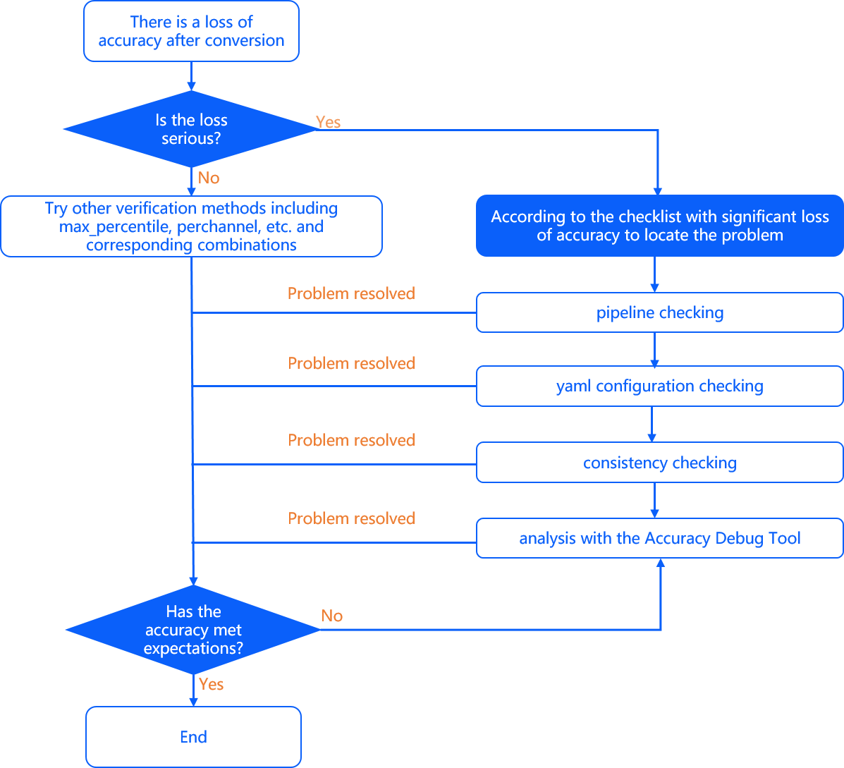
Based on previous accuracy analysis results, the accuracy loss problem of quantized model can be divided into the following 2 types:
1.There are apparent accuracy losses (over 4%).
This can be mostly caused by either inappropriate yaml configurations or unbalanced calibration datasets, etc. Please troubleshoot according to the following advices.
2.Accuracy loss is small (1.5%~3%).
If there are still small accuracy losses after the above cause is excluded, it is usually caused by model sensitivity and can be optimized using our accuracy optimization tool.
3.After trying 1 and 2, if the accuracy still does not meet expectations, try further attempts using the accuracy debug tool we provide.
The workflow chart of accuracy loss solution is shown as below:
First. Apparent Accuracy Loss (Over 4%)
Apparent accuracy loss are usually caused by all types of improper configurations, therefore, we suggest that you doublecheck the pipeline, model conversion configurations and consistency.
Doublecheck The Pipeline :
Pipeline refers to the entire process of data preparations, inference, post-processing and the accuracy evaluation Metric. Based on the past customer problem follow-up experiences, we find out that the most commonly seen case is that the modifications in the floating-point model training stage are not updated timely to the accuracy validation process during model conversion stage.
Doublecheck The Model Conversion Configurations :
As the
input_type_rtandinput_type_trainparameters are used for distinguishing the data formats of the converted heterogeneous model and the original floating-point model, it must be carefully doublechecked if they can meet the expectation, especially the sequences of BGR and RGB channels.Doublecheck if the
norm_type,mean_valuesandscale_valuesparameters are specified correctly. Nodes of the mean and scale operations can be directly inserted into the model by specifying the conversion configurations, and it should be confirmed whether repeated mean or scale operations are executed in the validation/evaluation images. Repeated pre-processing operation is another frequently-seen mistake.
Doublecheck Data Processing Consistency :
The
skimage.readandopencv.imreadare 2 popular image-reading methods, while there are differences in the output ranges and formats between the 2 methods. When using theskimageto read images, you can get RGB channel sequence, value ranges between 0~1 and float data type; but when using theopencv, you will get BGR channel sequence, value ranges between 0~225 and uint8 data type.We often use numpy’s tofile to serialize data during the calibration data preparation phase, when preparing application samples for an application. This approach does not save the shape and type information, which needs to be specified manually at load time, and requires you to ensure that the data type, data size, and data layout of the serialization and deserialization process of these files are consistent.
It is recommended that you still use the data processing libraries that the original floating-point model relied on during the training and validation phase of the D-Robotics toolchain. For less robust models, typical functions implemented in different libraries such as resize, crop, etc. may affect the model accuracy.
Validate if datasets are reasonably distributed. The volume of validation dataset should be around 100 and images should cover all scenarios. For example, in cases of multi-task and multi-class classification, the validation dataset should be able to cover all prediction branches or all classes. Meanwhile, try not to use those exceptional images (e.g. the over-exposed).
Use the *_original_float_model.onnx model to re-validate model accuracy. Normally, the accuracy of the *_original_float_model.onnx should be accurate to 3~5 decimal places. If your model fails to satisfy this accuracy, please carefully check the data processing.
Second. Improve Model Accuracy When There Is Smaller Accuracy Loss
In general, to reduce the difficulty of model accuracy optimization, we recommend that you use the automatic parameter search function in the conversion configuration. If you find that the accuracy results of the automatic search still fall short of expectations, the accuracy loss compared with the original floating-point model is in the range of 1.5% to 3%. You can try to improve the accuracy using the following suggestions respectively.
Try to manually specify the
calibration_type, you can selectmixfirst, if the final accuracy still does not meet expectations, then try eitherklormax.Try to enable the
per_channelparameter.When the
calibration_typeis specified asmax, try to specify themax_percentileinto0.99999,0.99995,0.9999,0.9995and0.999respectively.
Third. Accuracy Debug Tool
After trying the methods provided in I and II, if your accuracy still does not meet your expectations, we provide the accuracy debug tool to assist you in locating the problem for your convenience. This tool can help you analyze the quantified error at the node granularity of the calibration model and quickly locate nodes with accuracy anomalies. For a detailed description of the tool and how to use it, you can refer to section Accuracy Debug Tool .
Based on past practical production experience, the above strategies have been able to handle a variety of practical problems.
4.1.1.8.3. Further Improve Model Accuracy Using the QAT Solution
If the above analysis does not reveal any configuration problems, but the accuracy still cannot meet the requirements, it may be a limitation of PTQ itself. In such case, you can utilize the QAT solution to quantize the model.
This section elaborates the QAT Solution as follows:
Firstly, the About Quantization subsection introduces the concept and 2 different methods of quantization.
Secondly, the About Model Conversion subsection tells you what is D-Robotics’ model conversion all about, what is the original floating-point model and what is a heterogeneous model.
Thirdly, based on the understanding of the above-mentioned concepts, the About Model Quantization & Compilation subsection tells you more about the relationship between PTQ and QAT, so that you can choose an appropriate solution based on your own conditions;
Finally, the QAT Model Quantization & Compilation subsection introduces you how to complete the compilation of quantitative models through the QAT solution.
4.1.1.8.3.1. About Quantization
Most of the models currently trained on GPUs use floating-point number representation, i.e., model parameters are stored using floating-point numbers. D-Robotics’ Algorithm computing platform based on the BPU architecture are using the INT8 number (common precision for computing platforms in the industry) representation, they can support quantized model using the fixed-point number representations. The very process of converting the model using floating-point parameters into the model using fixed-point parameters is what we call quantization.
There are 2 quantization methods:
PTQ (Post Training Quantization) :
Firstly train a floating-point model, and then calculate the quantization parameters using calibration images. Finally, convert the floating-point model into the quantized model. This method is easier and faster, but there must be inevitable quantization loss.
Note
The quantization and compilation process of the PTQ model can be found in Model Quantization and Compilation .
QAT (Quantization Aware Training) :
The floating-point model structure is intervened first at the time of floating-point training to increase the quantization error, allowing the model to perceive the loss due to quantization. This method requires users retraining on the full training set and can effectively reduce the quantization error of quantization deployment. The QAT solution is a popular solution among many open source frameworks, e.g., The Eager Mode and FX Graph solutions of PyTorch, the tf-lite solution, etc.
Note
What is the relationship between QAT and floating-point training
QAT training is a finetune method, and it is best to use the QAT solution to improve the quantization accuracy when the floating-point results have been fitted. That is, the training contains two steps: firstly, train the floating-point model, till you’re satisfied with the model accuracy, and then use QAT to further improve the quantization accuracy.
To enable the model to better aware the quantization error, QAT are required to use the full volume training set. The number of epoch is related to the difficulty level of your model, approximately the epoch number should equal to 1/10 of the original floating-point training. Since the finetune is performed on a floating-point model, the learning rate of QAT training tries to be consistent with the last few epochs of the floating-point model.
4.1.1.8.3.2. About Model Conversion
Model conversion refers to the very process of converting the original floating-point model into heterogeneous model supported by D-Robotics. The process consists of pre-process node modification, original model graph optimization, model quantization and model compilation in dev board, etc.
The floating-point Model (also referred to as floating-point model in some parts of the text) is the available model that you get from training with DL frameworks such as TensorFlow/PyTorch, etc. This model has a computational accuracy of float32. Currently in our QAT solution, the training tool is developed based on Pytorch, so only models in Pytorch format are supported. The PTQ solution only supports Caffe & ONNX model formats, so for models in formats such as TensorFlow/PyTorch, they need to be quantized & compiled by D-Robotics’ tools by converting to ONNX models first.
The heterogeneous model is a model format suitable for running on D-Robotics computing platforms. It is called heterogeneous model because it can support model execution on both ARM CPU and BPU. Since the operation speed on the BPU will be much faster than that on the CPU, the operators will be computed on the BPU as much as possible. For operators that are not supported on the BPU at the moment, they will be computed on the CPU.
4.1.1.8.3.3. About Model Quantization & Compilation Workflow
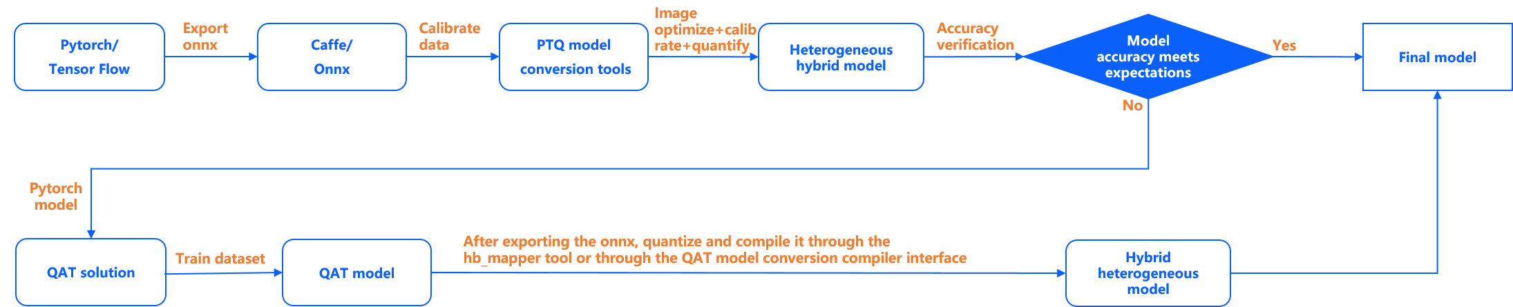
The following displays a normal workflow of model quantization and compilation:
Tip
It is recommended that users first try this method for model quantization compilation. In case the model accuracy cannot satisfy your requirement after PTQ and optimization, please try out the QAT solution instead.
4.1.1.8.3.4. QAT Model Quantization & Compilation Introduction
The D-Robotics Plugin Pytorch (hereinafter referred to as Plugin) refers to the official PyTorch quantization interface and ideas. The Plugin adopts the Quantization Aware Training (QAT) solution, so users are recommended to read the PyTorch official documentation related to the QAT.
For a more detailed introduction to D-Robotics Plugin Pytorch, you can refer to the Quantized Awareness Training (QAT) section.