6.1. PTQ Conversion Principle and Process
6.1.1. Overview
The process of the model from training to conversion to running on the development board is shown below:
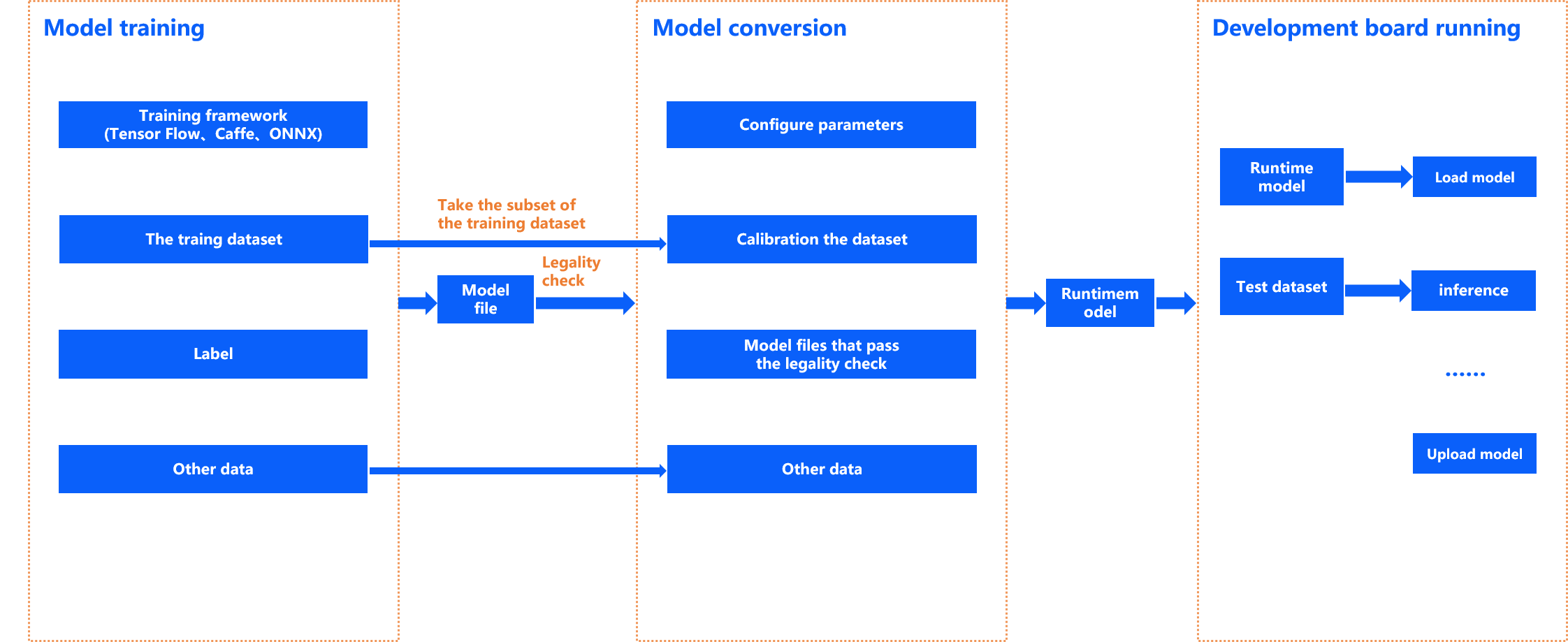
Model Training: It is the process of getting a usable model by using public deep learning frameworks such as TensorFlow, PyTorch, Caffe, etc. The trained model will serve as the input for the model conversion stage. The toolchain does not provide training-related libraries or tools. For the detailed supported public learning frameworks, please refer to the instructions in the Floating-point Model Preparation .
Model Conversion: Taking the floating-point model obtained from model training as input, this stage transforms floating-point models into hybrid heterogeneous models that can run efficiently on the D-Robotics computing platform through important steps such as model structure optimization and model calibration quantification. For more information, please refer to Model Quantization and Compilation section.
Embedded Application development: The toolchain supports application development in both X86 emulation environment and real embedded environment. In case you are not convenient to use the development board, you can debug the program and verify the calculation results in the emulation environment. In order to reduce the cost of simulation verification, the toolchain provides the exact same simulation library interface as the embedded interface, only with different compilation configurations. For more information, please refer to Embedded Application Development section.
Operator development: This stage is optional and it mainly solves the situation when the model has toolchain that does not support the operator. If you do not encounter such a situation, you can simply ignore this section. For more information, please refer to Custom OP Development section.
6.1.2. PTQ Conversion Process
Model conversion is the process of converting the original floating-point model to a D-Robotics hybrid heterogeneous model.
The original floating-point model (also referred to as a floating-point model in sections of the document) is an available model trained by a DL framework such as TensorFlow/PyTorch, with computation precision of float32; the hybrid heterogeneous model is a model format suitable for running on the D-Robotics computing platform.
This section will repeatedly use the two model terms. To avoid ambiguity, please understand the concept before reading the following section.
The complete the model development process with the D-Robotics toolchain involves five important stages: Floating-point Model Preparation, Model Verification, Model Conversion, Performance Evaluation, and Accuracy Evaluation, as shown in the figure below.
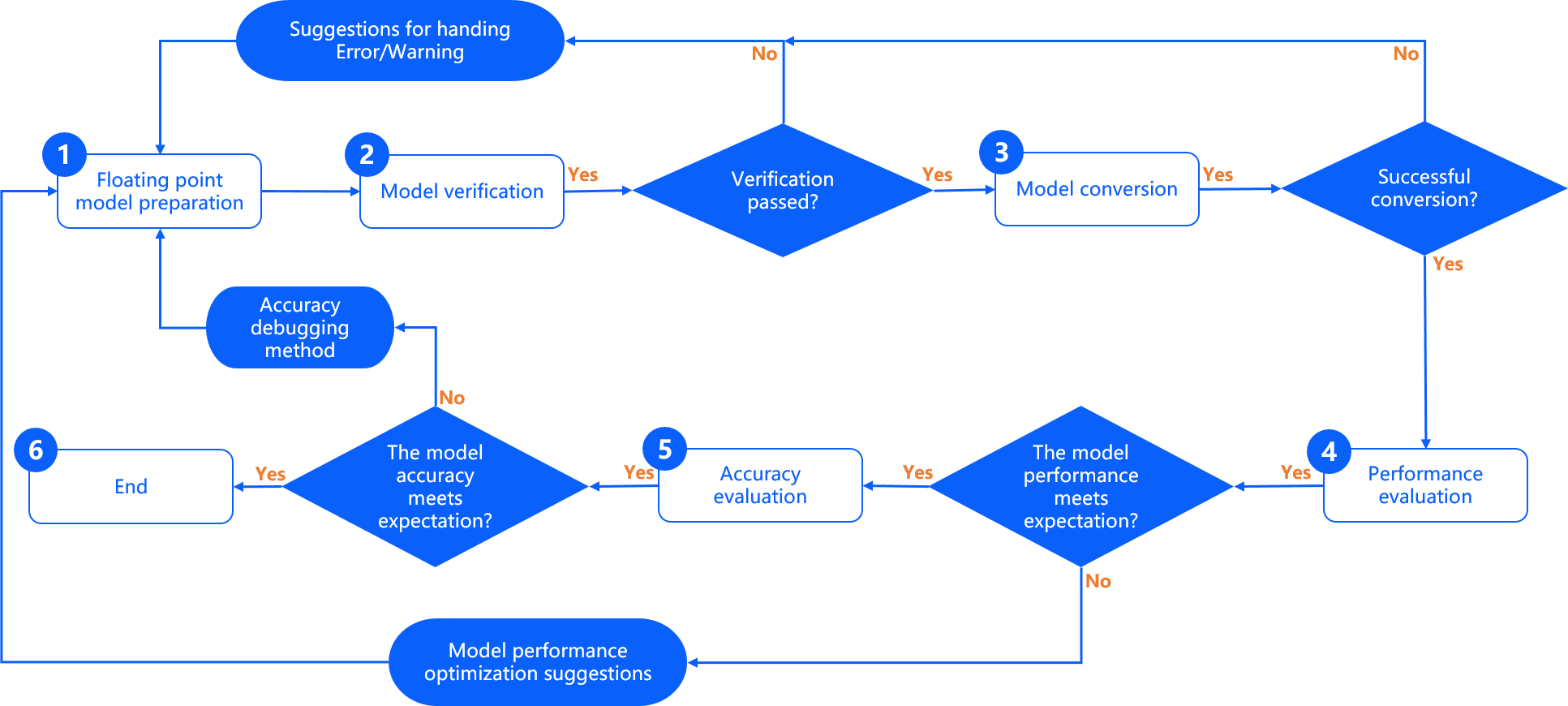
The Floating-point model, as the output of the Floating-point Model Preparation stage, will serve as the input of the model conversion tool. The floating-point model is usually trained on basis of some open source deep learning frameworks. Note that the model must be exported to a format supported by D-Robotics. For more information, please refer to the Floating-point Model Preparation.
The Model Verification stage is used to ensure that the model is computing platform compliant. D-Robotics provides specified tools to complete model validation, and for non-compliance, such tools will explicitly give you the specific operator information for the non-compliance, so that you can easily adjust the model with the description of the operator constraints. For more information, please refer to the Model Checking.
The Model Conversion stage converts the floating-point model to the hybrid heterogeneous model supported by D-Robotics. To run models efficiently on the D-Robotics computing platform, critical steps such as model optimization, quantization, and compilation are completed by D-Robotics’s model conversion tools. D-Robotics’s model quantization method has undergone long-term technological and production validation, and can guarantee an accuracy loss of less than 1% on most typical deep learning models. For more details about model conversion please refer to the Prepare Calibration Data and Model Quantization and Compilation.
The Performance Evaluation stage contains a series of tools to evaluate the model performance. Before deploying your application, you can use these tools to verify that the model performance meets application requirements. For some cases where the performance is not as good as expected, you can optimize the models based on D-Robotics’s model performance optimization advices. For more information, please refer to the Model Performance Analysis.
The Accuracy Evaluation stage contains a series of tools to evaluate the accuracy of the model. In most cases, D-Robotics’s converted-models can maintain almost the same accuracy as the original floating-point model. Before application deployment, you can use these tools to verify that the accuracy of the model meets the expectations. For some cases where the accuracy is not as good as expected, you can optimize the models based on D-Robotics’s model accuracy optimization advices. For more information, please refer to the Model Accuracy Analysis.
Attention
In general, you can get a qualified runtime model after model conversion. However, make sure that the performance and accuracy of the model are in line with the application requirements. D-Robotics strongly suggest you that each conversion shall be followed by the evaluation steps of performance and accuracy.
The model conversion process will generate onnx models, which are intermediate products and only facilitate users to verify the accuracy of the model. Therefore, the compatibility between versions is not guaranteed. When using the evaluation script in the example to evaluate the onnx model in a single image or on a test set, please use the onnx model generated by the current version of the tool.
6.1.3. Model Conversion Process Detailed Explanation
So how to convert the floating-point models trained by using the opensource ML frameworks (such as Caffe, TensorFlow, PyTorch, etc.) to the D-Robotics hardware supported fixed-point models?
In most cases, the threshold values and weights of the floating-point models obtained from either the opensource ML frameworks or trained by yourself are floating-point numbers (float32) and each number occupies 4 bytes.
However, by converting the floating-point numbers to fixed-point numbers (int8), each number occupies only 1 byte, thus the computation operations in the embedded runtime can be dramatically reduced.
Therefore, it brings significant performance boost by converting the floating-point models to fixed-point models with no loss or very small loss.
Typically, model conversion can be divided into the following steps:
1.Check if there are unsupported OPs in the models to be converted.
2.Prepare 20~100 images for calibration use at the conversion stage.
3.Convert the floating-point models to fixed-point models using the floating-point conversion tools.
4.Evaluate the performance and accuracy of the converted models to ensure that there isn’t huge difference in model accuracy before and after the conversion.
Run models in simulator/dev board to validate model performance and accuracy.
6.1.3.1. Model Checking (hb_mapper checker)
Note
If you need to do this process in the sample folder, you need to execute the 00_init.sh script in the folder first to get the corresponding original model and dataset.
Before converting the floating-point models into the fixed-point models,
we should check if there are D-Robotics hardwares unsupported OPs in the floating-point models using the hb_mapper checker tool.
If yes, the tool will report the unsupported OP(s).
Usage of the hb_mapper checker tool please refer to the section Model Checking Tool (hb_mapper checker) .
If unsupported ops are found during the process, it will prompt as follows:
ERROR HorizonRT not support these cpu operators: {name of the unsupported OP}
Tip
More information about D-Robotics hardware supported OPs, refer to Toolchain Operator Support Constraint List.
The tool will print out an OP list which also shows the running location of these ops, on the CPU or BPU. If the validation ends without error, you can proceed to the next step, as follows:
hb_mapper checker --model-type caffe --proto mobilenet_deploy.prototxt \
--model mobilenet.caffemodel --march bayes-e
2023-12-06 17:33:53,117 INFO log will be stored in ....
2023-12-06 17:33:53,117 INFO Start hb_mapper....
...
2023-12-06 17:33:53,118 INFO hb_mapper version 3.0.3
...
fc7          BPU  id(0)     HzSQuantizedConv
prob         CPU  --        Softmax
2023-12-06 17:33:53,329 INFO End to D-Robotics NN Model Convert.
2023-12-06 17:33:53,332 INFO ONNX model output num : 1
2023-12-06 17:33:53,351 INFO End model checking....
Tip
If unsupported op exists, you can either contact D-Robotics technical staff for the op development plan or refer to Custom OP Development section to add the OP via the Custom OP function.
6.1.3.2. Calibration Image Preparation
Note
If you need to do this process in the sample folder, you need to execute the 00_init.sh script in the folder first to get the corresponding original model and dataset.
When converting the floating-point models, you need to prepare 20~100 images for calibration use at the calibration stage.
Input image formats may vary by input type and layout. In this stage, because both original (JPG, etc.) and the processed images are valid, you can either feed the calibration images used in the model training or feed your own processed images.
We recommend you preprocessing the calibration images on your own: Firstly, complete the operations such as image channel (BGR/RGB), data layout (NHWC/NCHW), and image resizing/padding (Resize&Padding). Secondly, set preprcess_on to False in the YAML file (i.e., mobilenet_config.yaml). The tool will then feed the images to the calibration stage after loading them as binary files.
Taking MobileNet as an example, the required transformer operations are as follows:
transformers = [
      ShortSideResizeTransformer(short_size=256),   # Pad the short side to 256 to maintain length-width ratio
      CenterCropTransformer(crop_size=224),         # Crop a 224\*224 image from the center of the image
      HWC2CHWTransformer(),                         # Switch data layout from NHWC to NCHW
      RGB2BGRTransformer(data_format="CHW"),        # Switch color channel from RGB to BGR
      ScaleTransformer(scale_value=255),            # Switch number range from 0-1 to 0-255
  ]
Tip
If the color space in model training is BGR/RGB, then the color space of those images that will pass to the tool at the calibration stage must also be BGR/RGB. The tool can convert the color from BGR/RGB to YUV444/Gray automatically.
For example, in the above code block, the actual input of the MobileNet model is specified as NV12, but after 02_preprocess.sh conversion, the color space will be switched to BGR, and the remaining conversion from BGR to NV12 are automatically done by the tool.
6.1.3.3. Model Conversion (hb_mapper makertbin)
When you confirm that the floating-point model can be successfully converted by using the hb_mapper checker tool,
you can then convert the floating-point model to a D-Robotics hardware supported fixed-point model by using the hb_mapper makertbin tool.
This tool requires you to pass in the type ( caffe / onnx ) of the model for conversion as well as a configuration file (*.yaml) containing conversion requirements.
For specific configuration file settings and the insturctions of each parameter, refer to the descriptions in sections Specific Parameter Information and Configuration File Template .
When the model conversion process ends, it also prints the level of similarity between the floating-point model and fixed-point model to the log, you can therefore judge the similarity before and after conversion according to the Cosine Similarity field.
As shown in the example below, the value of Cosine Similarity is very close to 1, so the performance of the fixed-point model should be very close to that of the floating-point model before the conversion.
2023-12-06 20:26:50,149 INFO Start hb_mapper....
......
2023-12-06 20:27:21,427 INFO End to compile the model with march bayes-e.
2023-12-06 20:27:21,429 INFO The converted model node information:
======================================================================================================================
Node                    ON   Subgraph  Type                           Cosine Similarity  Threshold   In/Out DataType
----------------------------------------------------------------------------------------------------------------------
HZ_PREPROCESS_FOR_data  BPU  id(0)     HzSQuantizedPreprocess         0.999988           127.000000  int8/int8
conv1                   BPU  id(0)     HzSQuantizedConv               0.999922           2.937425    int8/int8
conv2_1/dw              BPU  id(0)     HzSQuantizedConv               0.999378           2.040827    int8/int8
conv2_1/sep             BPU  id(0)     HzSQuantizedConv               0.996680           4.486579    int8/int8
conv2_2/dw              BPU  id(0)     HzSQuantizedConv               0.997340           3.545496    int8/int8
conv2_2/sep             BPU  id(0)     HzSQuantizedConv               0.996384           2.791299    int8/int8
conv3_1/dw              BPU  id(0)     HzSQuantizedConv               0.994165           1.417208    int8/int8
conv3_1/sep             BPU  id(0)     HzSQuantizedConv               0.985451           2.188753    int8/int8
conv3_2/dw              BPU  id(0)     HzSQuantizedConv               0.994921           1.822225    int8/int8
conv3_2/sep             BPU  id(0)     HzSQuantizedConv               0.994251           1.841765    int8/int8
conv4_1/dw              BPU  id(0)     HzSQuantizedConv               0.988263           1.043535    int8/int8
conv4_1/sep             BPU  id(0)     HzSQuantizedConv               0.990294           1.736999    int8/int8
conv4_2/dw              BPU  id(0)     HzSQuantizedConv               0.992460           0.990603    int8/int8
conv4_2/sep             BPU  id(0)     HzSQuantizedConv               0.993468           1.574677    int8/int8
conv5_1/dw              BPU  id(0)     HzSQuantizedConv               0.988949           0.823123    int8/int8
conv5_1/sep             BPU  id(0)     HzSQuantizedConv               0.990803           1.265912    int8/int8
conv5_2/dw              BPU  id(0)     HzSQuantizedConv               0.990202           0.772344    int8/int8
conv5_2/sep             BPU  id(0)     HzSQuantizedConv               0.983443           1.530479    int8/int8
conv5_3/dw              BPU  id(0)     HzSQuantizedConv               0.986502           0.783812    int8/int8
conv5_3/sep             BPU  id(0)     HzSQuantizedConv               0.977642           1.927324    int8/int8
conv5_4/dw              BPU  id(0)     HzSQuantizedConv               0.982337           0.996043    int8/int8
conv5_4/sep             BPU  id(0)     HzSQuantizedConv               0.962062           2.167391    int8/int8
conv5_5/dw              BPU  id(0)     HzSQuantizedConv               0.978872           1.923361    int8/int8
conv5_5/sep             BPU  id(0)     HzSQuantizedConv               0.960184           3.578415    int8/int8
conv5_6/dw              BPU  id(0)     HzSQuantizedConv               0.980317           2.463874    int8/int8
conv5_6/sep             BPU  id(0)     HzSQuantizedConv               0.981055           4.124151    int8/int8
conv6/dw                BPU  id(0)     HzSQuantizedConv               0.998241           0.667692    int8/int8
conv6/sep               BPU  id(0)     HzSQuantizedConv               0.985220           0.983833    int8/int8
pool6                   BPU  id(0)     HzSQuantizedGlobalAveragePool  0.993602           11.415899   int8/int8
fc7                     BPU  id(0)     HzSQuantizedConv               0.995105           5.843800    int8/int32
prob                    CPU  --        Softmax                        0.985517           --          float/float
2023-12-06 20:27:21,430 INFO The quantify model output:
=======================================================================
Node  Cosine Similarity  L1 Distance  L2 Distance  Chebyshev Distance
-----------------------------------------------------------------------
prob  0.985517           0.000385     0.000203     0.185123
2023-12-06 20:27:21,432 INFO End to D-Robotics NN Model Convert.
Note
The CosineSimilarity in the log refers to the very first image in the calibration images, it cannot fully represent the model accuracy before and after the conversion.
After the model conversion, the following files will be generated under the folder model_output (default name):
\*_subgraph_0.html: Static performance evaluation file (with better readability)\*_subgraph_0.json: Static performance evaluation file\*_original_float_model.onnx: Original floating-point model (floating-point model)\*_optimized_float_model.onnx: Optimized floating-point model\*_calibrated_model.onnx: Calibration model\*_quantized_model.onnx: Fixed-point model\*.bin: Hybrid model to run in dev board
These model files are the output of the conversion at key stages and will be used in the subsequent steps.
Note
You can use the
03_classification/01_mobilenet/mapper/03_build.shscript to experience thehb_mapper makertbintool.If you want to learn more about the model conversion workflow, please read Model Quantification and Compilation.
6.1.3.4. Single Image Inference
The accuracy of the fixed-point model generated by the floating-point conversion must be evaluated.
You should have good understanding of the input/output structures of the model. You should also be able to accurately preprocess the input images of the model, postprocess the model outputs, and write the model execution scripts on your own.
You can refer to the sample code in 03_classification/01_mobilenet/mapper/04_inference.sh in D-Robotics model conversion sample package.
The code logic of the model accuracy validation are as follows:
import numpy as np
# Load D-Robotics dependency library
from horizon_tc_ui import HB_ONNXRuntime
from postprocess import postprocess

# Prepare the input for model running, here the `input.py` is the processed data
input_data = np.load("input.npy")
# Load model file
sess = HB_ONNXRuntime(model_file = "***_quantized_model.onnx")
# Obtain the model input & output node information
input_names = sess.input_names
output_names = sess.output_names
# Prepare the input data, here we assume the model has only one input
input_info = {input_names[0]: input_data}
# Model inference, the return value is a list that corresponds in order to the names specified by output_names
output = sess.run(output_names, input_info)
# Postprocessing
top_five_label_probs = postprocess(output)
As shown above, this single image inference script is used for validating model accuracy by inferencing a zebra image.
After preprocessing the image data from RGB to the intermediate type of input_type_rt (no -128 required). As input_type_rt of the example mobilenet is NV12, the corresponding intermediate type is YUV444_128, the infer_transformers` process needs to complete the conversion of RGB–>NV12–>YUV444. For informaiton about intermediate types, refer to the Model Conversion Interpretation.
Then, infer the model by passing the above image data by using the HB_ONNXRuntime command, post-processing after inference, and finally print out 5 of its most likely types.
The output of the script is shown as follows with the most possible class being label: 340:
I0108 18:11:47.398328 140427646048000 cls_inference.py:89] The input picture is classified to be:
label 340: prob 0.97
label 292: prob 0.02
label 282: prob 0.00
label 83: prob 0.00
label uses the ImageNet label classes, you can also find it in the 01_common/test_data/classes.txt file in the D-Robotics Model Conversion Sample Package, where the corresponding class of 340 is zebra, so the inference result is correct.
6.1.3.5. Model Performance Evaluation
One of the important performance indicators is the frame rate of a model running on the dev board.
To save developers from setting up a dev board environment, you can use the hb_perf tool to analyze the performance of the fixed-point model.
In the MobileNetv1 sample, after running the hb_perf mobilenetv1_224x224_nv12.bin command, you can find the model analysis file mobilenetv1_224x224_nv12.html under hb_perf_result/mobilenetv1_224x224_nv12/, as follows:
[horizon@gpu-dev model_output]$ hb_perf mobilenetv1_224x224_nv12.bin
2023-12-06 19:40:21,305 INFO log will be stored in horizon/.../mobilenetv1/hb_perf.log
2023-12-06 19:40:21,322 INFO Start hb_perf....
2023-12-06 19:40:21,323 INFO hb_perf version 1.21.0
2023-12-06 19:40:21,375 INFO ********* mobilenetv1_224x224_nv12 perf **********
......
2023-12-06 19:40:21,875 INFO file stored at : horizon/.../mobilenetv1_224x224_nv12/mobilenetv1_224x224_nv12.html
In mobilenetv1_224x224_nv12.html, we can see the overall model performance data.
When a model contains more than one segment, an individual performance analysis report on each segment running on the BPU will be generated.
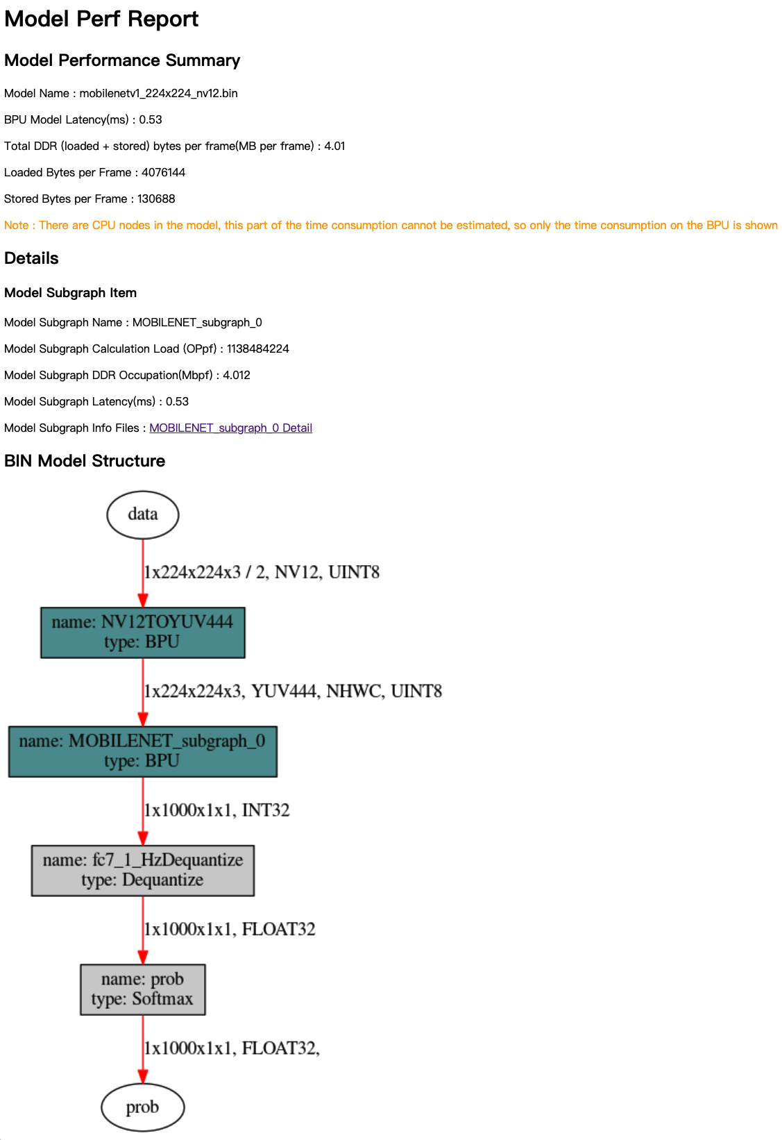
Performance indicators in the above graph are explained as follows:
Model Name: Model name.BPU Model Latency(ms): overall time consumption of the model (unit: ms).Total DDR (loaded+stored) bytes per frame(MB per frame): Total amount of DDR space occupied by data loading and storage of the BPU part of the model (unit: MB/frame).Loaded Bytes per Frame: Loaded bytes per frame at the model runtime.Stored Bytes per Frame: Stored bytes per frame at the model runtime.
Note
The above BPU Model Latency(ms) refers to the time taken by the part of model to run on the BPU; However, the time taken by the part of the model that runs on the CPU, if there is any, is not counted.
6.1.3.6. Model Accuracy Evaluation
It’s insufficient to determine the model accuracy by single image inference, so you still need to use scripts to evalute the model accuracy after the conversion.
To do so, you need some coding work to enable the model to loop the image inference and compare the inference results with standard results to get model accuracy results.
In model accuracy evaluations, images must be pre-processed and the model output must be post-processed, so here we provide a Python script as a sample.
The logic of this script is the same as that of single image inference, yet it must run on the entire dataset.
The script can evaluate the model output results and generate evaluation results.
Because it takes a long time to run the script, you can set the number of threads to run the evaluation by specifying the PARALLEL_PROCESS_NUM environment variable.
The output of the script is shown as follows:
===REPORT-START{MAPPER-EVAL}===
0.7011
===REPORT-END{MAPPER-EVAL}===
As you can see that the accuracy of the converted fixed-point model is 0.7011.
Note
Model accuracy may vary slightly due to the differences of operating systems and dependencies.
Model accuracy may vary slightly by iteration.
If you find that there is an accuracy loss after model conversion, please visit the D-Robotics Developer Community.
6.1.3.7. [Reference] Supported Calibration Methods
We currently support the following calibration methods:
1.Default
Default is a strategy that automatically searches the calibrated quantization parameters to obtain a relatively good combination.
2.Mix
Mix is a search strategy that integrates multiple calibration methods, which automatically identifies quantization-sensitive nodes, selects the best from a group of calibration methods at node granularity, and finally build a hybrid calibration method absorbing the advantages of multiple calibration methods.
3.KL
KL learns from the Solution proposed by TensorRT, uses the KL entropy value to traverse the data distribution of each quantized layer, and determines threshold value by searching for the lowest KL entropy value.
As this method can cause more data saturation and smaller data quantization granularity, it more suitable than max for those neural network models with more concentrated data distribution.
4.Max
Max refers to a calibration method that automatically selects the max value in quantized layer as the threshold.
This method can cause oversized quantization granularity; however, it also causes less saturated points than the KL method, which makes it suitable for those neural network models with more discrete data distribution.
5.Load
This parameter is required when using the model exported by QAT.
6.Skip
If the model performance is the only concern without precision requirements, you can try the skip calibration method,
which uses max + internally generated random calibration data for calibration and does not require you to prepare calibration data,
so it is more suitable for the first attempts to validate the model structure.
Attention
As the skip method uses max + internally generated random calibration data for calibration, the model obtained cannot be used for accuracy verification.
6.1.3.8. [Reference] OP List
For more information about the operators and corresponding constraints currently supported by D-Robotics Algorithm Toolchain, please refer to Toolchain Operator Support Constraint List.