3.2. Algorithm Model PTQ + On-board Deployment Quick Start¶

To help you quickly get started, this section introduces the basic workflow of the PTQ scheme using MobileNet-v1 as an example to illustrate the details.

The basic workflow is as follows:

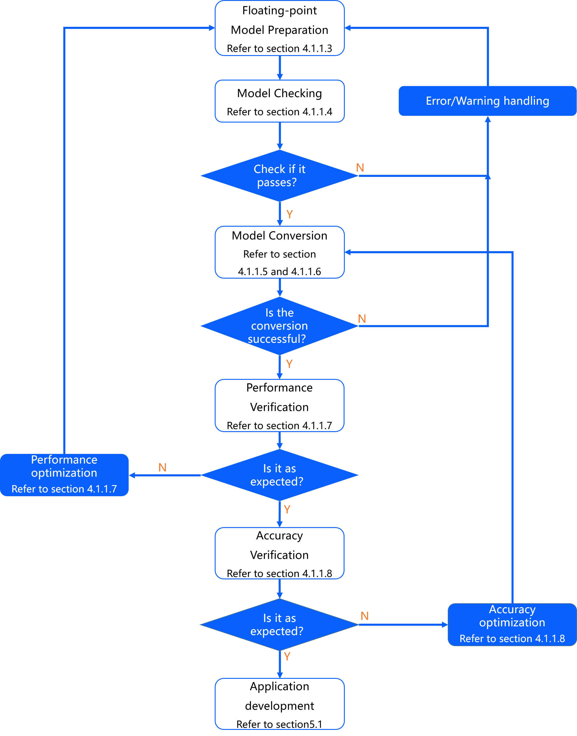
Attention

Before starting, make sure you have completed the environment installation on both dev PC and dev board by following the section Environment Deployment.

3.2.1. Floating-point Model Preparation¶

The OE package provides you with rich PTQ model samples under the ddk/samples/ai_toolchain/horizon_model_convert_sample path. The MobileNet-v1 model sample is located under the 03_classificarion/01_mobilenet path.

Please first execute the 00_init.sh script to obtain the corresponding calibration dataset and the original model of the sample. Please refer to section Preparing Models for their model sources and related instructions.

If you need to convert a private model, refer to section Floating-point Model Preparation to prepare caffe1.0 or opset=10/11 onnx models in advance. The following table shows reference schemes for converting different frameworks to ONNX model formats.

Training Framework	Reference Scheme
Pytorch	Export using the official API. https://pytorch.org/tutorials/advanced/super_resolution_with_onnxruntime.html
Tensorflow	Convert using the ONNX community’s onnx/tensorflow-onnx tool. https://github.com/onnx/tensorflow-onnx
PaddlePaddle	Export using the official API. https://www.paddlepaddle.org.cn/documentation/docs/en/api/paddle/onnx/export_en.html
MXNet2Onnx	Export using the official API. https://github.com/dotnet/machinelearning/blob/main/test/Microsoft.ML.Tests/OnnxConversionTest.cs
Other frameworks	https://github.com/onnx/tutorials#converting-to-onnx-format

3.2.2. Model Verification¶

After the floating-point model is ready, we recommend a quick verification of the model to ensure that it meets the support constraints of the computing platform. For the MobileNet-v1 model of the Caffe1.0 framework, we can complete the model verification by typing the following command in the command line:

hb_mapper checker --model-type caffe \
                  --proto mobilenet_deploy.prototxt \
                  --model mobilenet.caffemodel \
                  --march bernoulli2

For an Efficientnet_lite0 model in ONNX format, type the following command:

hb_mapper checker --model-type onnx \
                  --model efficientnet_lite0_fp32.onnx \
                  --march bernoulli2

Where both model files are available from the ddk/samples/model_zoo/mapper/classification path.

The main parameters of the hb_mapper checker tool are as follows, for more parameter descriptions, refer to section Model Checking.

Parameter	Description
--model-type	Used to specify the type of model to check the input, currently only Caffe or ONNX is supported.
--march	Used to specify the type of processor to be adapted, for X3 processor, please set to bernoulli2 (default value).
--proto	This parameter is only valid if model-type specifies Caffe, the value is the name of the prototxt file of the Caffe model. You do not need to specify it if your model is the ONNX model.
--model	When model-type is specified as Caffe, the value is the name of the caffemodel file of the Caffe model. When model-type is specified as ONNX, the value is the ONNX model file name.

Take the MobileNet-v1 model as an example, you can execute the 01_check.sh script to quickly complete model verification.

The main contents of the 01_check.sh script file are as follows:

set -ex
cd $(dirname $0) || exit
model_type="caffe"
proto="../../../01_common/model_zoo/mapper/classification/mobilenet/mobilenet_deploy.prototxt"
caffe_model="../../../01_common/model_zoo/mapper/classification/mobilenet/mobilenet.caffemodel"
march="bernoulli2"

hb_mapper checker --model-type ${model_type} \
                  --proto ${proto} --model ${caffe_model} \
                  --march ${march}

If the model validation fails, confirm the error messages and modification suggestions according to the hb_mapper_checker.log file printed on the terminal or generated under the current path, please refer to section Model Checking for more instructions.

3.2.3. Model Conversion¶

After the model is validated, you can use the hb_mapper makertbin tool to covert the model, refer to the following command:

hb_mapper makertbin --config mobilenet_config.yaml \
                    --model-type caffe

Among them, mobilenet_config.yaml is the configuration file corresponding to the model conversion, which is described in section Yaml Configuration File, and model-type is used to specify the model type to check the input, which can be configured as Caffe or ONNX, and the parameters of the configuration files will be slightly different for different model types.

In addition, the model quantification of the PTQ scheme also depends on a certain number of pre-processed samples for calibration, which is described in section Pre-processing Calibration Data.

3.2.3.1. YAML Configuration File¶

The YAML configuration file contains 4 required parameter groups (model_parameters, input_parameters, calibration_parameters, compiler_parameters) and 1 optional parameter group (custom_op), each parameter group contains both required and optional parameters (optional parameters are hidden by default), refer to the model example and the section Model Quantification and Compilation for specific requirements and filling methods.

The MobileNet-v1 model configuration file is as follows:

# Parameters related to model conversion
model_parameters:

  # Caffe floating-point network data model file
  caffe_model: 'mobilenet.caffemodel'

  # Caffe network description file
  prototxt: 'mobilenet_deploy.prototxt'

  # Applicable BPU architecture
  march: "bernoulli2"

  # Specify whether to output the intermediate results of each layer during the model conversion,
  # if True, output intermediate output results of all layers
  layer_out_dump: False

  # The directory where the output results of the model conversion are stored
  working_dir: 'model_output'

  # The name prefix of the model file generated by the model conversion and used for on-board execution
  output_model_file_prefix: 'mobilenetv1_224x224_nv12'

# Model input related parameters, if multiple nodes are entered, use ';' to separate them,
# or write None if you use the default settings
input_parameters:

  # (Optional) node name of model input,
  # it shall be the same as the name of model file, otherwise an error will be reported,
  # the node name of model file will be used when left blank
  input_name: ""

  # The data format input to the network when the network is actually executed,
  # including nv12/rgb/bgr/yuv444/gray/featuremap
  input_type_rt: 'nv12'

  # Input data format for network training, the optional values are rgb/bgr/gray/featuremap/yuv444
  input_type_train: 'bgr'

  # The input data layout for network training, with optional values NHWC/NCHW
  input_layout_train: 'NCHW'

  # (Optional)the input size of model network, seperated by 'x'
  # note that the network input size of model file will be used if left blank
  # otherwise it will overwrite the input size of model file
  input_shape: ''

  # the data batch_size to be passed into neural network when actually performing neural network, default value: 1
  #input_batch: 1

  # Preprocessing methods for network input, mainly the following:
  # no_preprocess Do not do any operation
  # data_mean Subtract the channel mean value mean_value
  # data_scale Multiply the image pixels by the data_scale factor
  # data_mean_and_scale Subtract the channel mean and then multiply by the scale factor
  norm_type: 'data_mean_and_scale'

  # The mean value of the image subtracted, if it is a channel mean, the values must be separated by spaces
  mean_value: 103.94 116.78 123.68

  # The image preprocessing scaling factor, if it is a channel scaling factor, the value must be separated by spaces
  scale_value: 0.017

# Model quantification related parameters
calibration_parameters:

  # The storage directory of reference images for model quantification,
  # the image format supports JPEG, BMP and other formats, the input images should be from typical scenes used,
  # usually 20~100 images are selected from the test set, and the input images should cover typical scenes,
  # not remote scenes, such as overexposed, saturated, blurred, pure black, pure white, etc.
  # If there are multiple input nodes, separate them by ';'
  cal_data_dir: './calibration_data_bgr'

  # Data storage type for calibration data binary files, optional values: float32, uint8. If there are multiple input nodes, separate them by ';'
  cal_data_type: 'float32'

  # The algorithm type of model quantization, support default, mix, kl, max, load, usually use default can meet the requirements.
  # If it does not meet the expectation, you can try to change it to mix first. If there is still no expectation, try kl or max again.
  # When using QAT to export the model, this parameter should be set to load.
  # For more details of the parameters, please refer to the parameter details in PTQ Principle And Steps section of the user manual.
  calibration_type: 'max'

  # This parameter is for the 'max' calibration method and is used to
  # adjust the intercept point for the 'max' calibration.
  # This parameter is only valid when calibration_type is 'max'.
  # The value range of parameter is 0.5 ~ 1.0.
  # Common configuration options are: 0.99999/0.99995/0.99990/0.99950/0.99900.
  max_percentile: 0.9999

# Compiler Related Parameters
compiler_parameters:

  # Compile policy, supports bandwidth and latency optimization mode;
  # bandwidth is to optimize the bandwidth of DDR access.
  # latency is to optimize the inference time
  compile_mode: 'latency'

  # The default value of debug is True, that means turnning on the debug mode of the compiler,
  # which can output information related to performance simulation,
  # such as frame rate, DDR bandwidth usage, etc.
  debug: True

  # Optimization level can be selected from O0 to O3
  # O0, not optimized, it is the lowest optimization level with the fastest compilation speed,
  # O1 to O3, as the optimization level increases, it is expected that the compiled model will execute faster,
  # but it will also take longer to compile.
  # O2 is recommended for the fastest verification
  optimize_level: 'O3'

In this case, instead of configuring the caffe_model and prototxt parameters in the model_parameters parameter group, the ONNX model is repleaced with the onnx_model parameters.

The input_type_rt and input_type_train parameters in the input_parameters parameter group are used to specify the data type (e.g., NV12) that the model will receive when it is actually deployed on the board and the data type (e.g., RGB) for its own training, respectively. When the two data types are inconsistent, the conversion tool automatically inserts a BPU-accelerated preprocessing node in the frontend of the model to complete the corresponding color space conversion.

Meanwhile, the norm_type, mean_value, and scale_value parameters in this parameter group can also be used to configure the data normalization operation of the image input model, which will be integrated into the preprocessing node for BPU acceleration by the conversion tool after configuration.

The formula for data normalization is as follows:

\(data\_norm = (data - mean\_value) * scale\_value\)

The cal_data_dir parameter in the calibration_parameters parameter group needs to be configured with the path of the preprocessed calibration data folder, refer to the section Pre-processing Calibration Data for the descriptions of the preprocessing method.

3.2.3.2. Pre-processing Calibration Data¶

Attention

Please note that before doing this step, make sure that you have already finished obtaining the calibration dataset by executing the 00_init.sh script in the corresponding sample directory.
If you are currently only concerned with model performance, you can configure the calibration_type parameter in the yaml file directly to skip and skip this subsection. The tool will automatically ignore the cal_data_dir parameter when the model is converted.

The calibration data of the PTQ scheme is generally screened from the training set or verification set of about 100 (can be appropriately increased or decreased) typical data, and should avoid very rare and unusual samples, such as solid color images, images without any detection or classification targets, etc.

The filtered calibration data should also needs to be preprocessed in the same way as that before the model inference, and after processing, the data type (input_type_train), layout (input_layout_train) and size (input_shape) should stay the same as the original model.

For the preprocessing of calibration data, D-Robotics recommends directly using and modifying the sample code. Take the MobileNet-v1 model as an example, the calibration_transformers function in the preprocess.py file contains the pre-processing transformers for its calibration data, and the processed calibration data is consistent with its YAML configuration file, that is:

input_type_train ： ‘bgr’
input_layout_train ：’NCHW’

def calibration_transformers():
    transformers = [
        ShortSideResizeTransformer(short_size=256),
        CenterCropTransformer(crop_size=224),
        HWC2CHWTransformer(),
        RGB2BGRTransformer(data_format="CHW"),
        ScaleTransformer(scale_value=255),
    ]
    return transformers

where transformers are defined in ../../../01_common/python/data/transformer.py file, please refer to section Image Processing Transformer. You can choose to modify and extend them as needed.

Attention

Note that if the mean_value and scale_value parameters have been configured in the yaml file to normalize the data to enable BPU acceleration, you should avoid repeating the operation in the transformers here.

After modifying the preprocess.py file, you can modify and execute the 02_preprocess.sh script to complete the preprocessing of the calibration data.

bash 02_preprocess.sh

The main contents of the 02_preprocess.sh script file is as follows:

set -e -v
cd $(dirname $0) || exit

python3 ../../../data_preprocess.py \
  --src_dir ../../../01_common/calibration_data/imagenet \
  --dst_dir ./calibration_data_bgr \
  --pic_ext .bgr \
  --read_mode skimage \
  --saved_data_type float32

The parameters of the data_preprocess.py file is described as follows:

src_dir: Path to the raw calibration data.
dst_dir: Storage path of the processed data, which can be customized.
pic_ext: File suffix of the processed data, which is mainly used to help remember the data type and can be left unconfigured.
read_mode: Image reading mode, which can be configured as skimage or opencv. Note that the format of the image read by skimage is RGB with the data range of 0-1, while the format of the image read by opencv is BGR with the data range of 0-255.
saved_data_type: Type of saved data after processing.

If you choose to write your own python code to pre-process the calibration data, you can use the numpy.tofile command to save it as a float32 format binary file, which will be read by the toolchain calibration based on the numpy.fromfile command.

3.2.3.3. Model Conversion¶

After preparing the calibration data and YAML configuration file, you can complete the entire process of model parsing, graph optimization, calibration, quantization, and compilation conversion in one command.

For a detailed explanation of the internal process, please refer to section Model Conversion Interpretation.

Taking the MobileNet-v1 model as an example, the model conversion reference command is as follows:

hb_mapper makertbin --config mobilenet_config.yaml \
                    --model-type caffe

After conversion, the model file produced at each stage and the static performance evaluation files of the model BPU part estimated by the compiler will be saved under the working_dir path configured in the YAML file. For details, refer to Interpret Conversion Output.

|-- MOBILENET_subgraph_0.html        # Static performance evaluation files (better readability)
|-- MOBILENET_subgraph_0.json        # Static performance evaluation files
|-- mobilenetv1_224x224_nv12.bin     # Models for loading and running on the D-Robotics computing platform
|-- mobilenetv1_224x224_nv12_calibrated_model.onnx
|-- mobilenetv1_224x224_nv12_optimized_float_model.onnx
|-- mobilenetv1_224x224_nv12_original_float_model.onnx
`-- mobilenetv1_224x224_nv12_quantized_model.onnx

3.2.4. Fast Performance Verification¶

For the xxx.bin model file generated by the conversion, D-Robotics supports both first estimating the static performance of the BPU part of the model on the dev PC first, and providing an executable tool on the board to quickly evaluate the dynamic performance without any coding.

For more detailed descriptions and performance tuning recommendations, refer to section Model Performance Analysis and Optimization.

3.2.4.1. Static Performance Evaluation¶

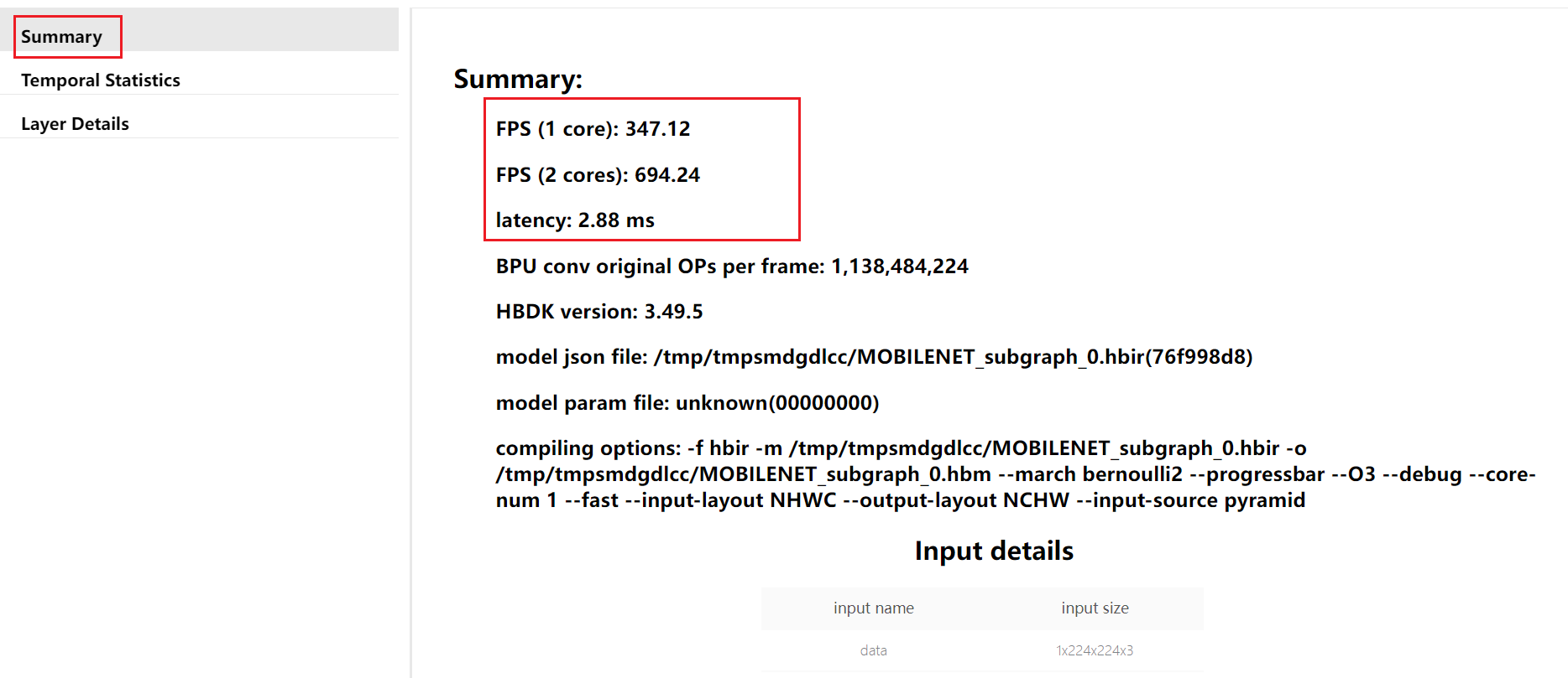
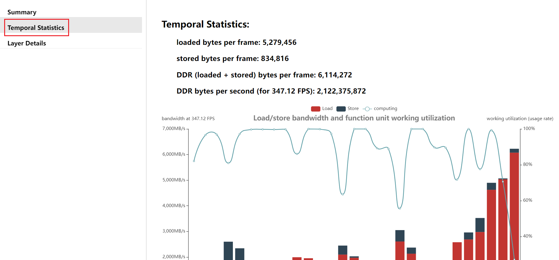
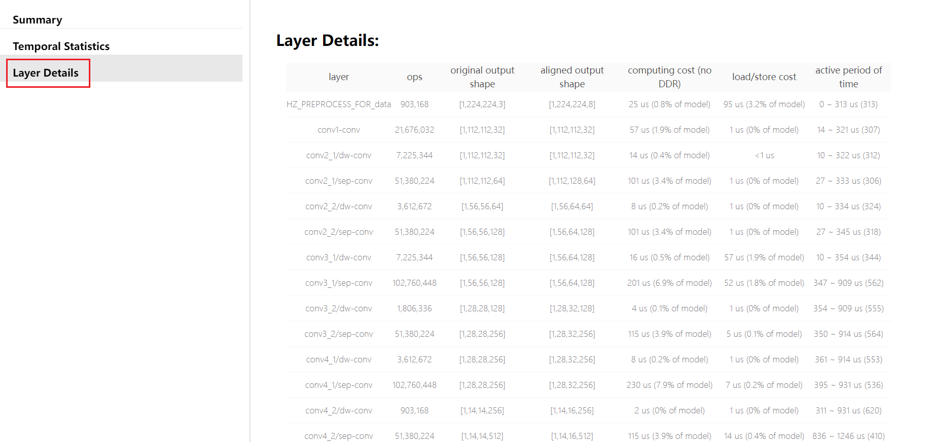
As described in section Model Conversion, after model conversion, HTML and JSON files containing static performance evaluation information for the model will be generated under the working_dir path, both with the same content. But the HTML file is more readable. The following is the HTML file generated by the MobileNet-v1 model conversion, where:

The Summary tab provides the performance of the BPU part of the model predicted by the compiler (excluding CPU operator performance prediction).

The Temporal Statistics tab provides the bandwidth usage of the model during the inference time of one frame.

../../../_images/temporal_statistics_tab.png

The Layer Details tab provides the computation amount, original op output shape, aligned op output shape, computation time, data handling time and the active time period of the compiled layer (does not represent the execution time of the layer, usually multiple layers alternate/execute in parallel) of each layer of BPU operators.

For the xxx.bin model, D-Robotics also provides the hb_perf tool in the dev PC environment to regenerate static performance prediction files.

For detailed instructions, refer to section Use The hb_perf Tool To Evaluate Model Performance.

The hb_perf tool is used as follows:

hb_perf xxx.bin

When the static performance of the model no longer meets expectations, refer to section Model Performance Optimization for performance tuning.

3.2.4.2. Dynamic Performance Evaluation¶

Once the static performance of the model meets expectations, we can further evaluate the dynamic performance of the model on the board, and the reference method is as follows:

1.Make sure you have completed the environment deployment of the dev board according to section Environment Deployment.

2.Copy the xxx.bin model generated by the conversion to any path in the /userdata folder of the dev board.

3.Use the hrt_model_exec perf tool to quickly evaluate the time consumption and frame rate of the model.

# Copy the model to the dev board
scp model_output/mobilenetv1_224x224_nv12.bin root@{board_ip}:/userdata

# Log in to the dev board to evaluate the performance
ssh root@{board_ip}
cd /userdata

# Evaluate the latency in the single-BPU core single-threaded serial state
hrt_model_exec perf --model_file mobilenetv1_224x224_nv12.bin --thread_num 1 --frame_count 1000

# Evaluate the FPS in the dual-BPU cores multi-threaded concurrent state
hrt_model_exec perf --model_file mobilenetv1_224x224_nv12.bin --core_id 0 --thread_num 8 --frame_count 1000

The main parameters of the hrt_model_exec tool are described as follows, refer to the section hrt_model_exec Tool Introduction for more instructions:

Parameter	Type	Description
model_file	string	[Required] Model file path
core_id	int	[Optional] Used to specify the BPU operation core, defaults to 0. 0: Arbitrary core, the prediction library will automatically allocate schedules according to the load. 1: core0. 2: core1.
thread_num	int	[Optional] Number of threads to run the program, optional range [1,8], defaults to 1.
frame_count	int	[Optional] Total number of frames the model runs, defaults to 200.
profile_path	string	[Optional] Statistical tool log generation path, run to generate profiler.log and profiler.csv, analyze op time and scheduling time consumption.

Note

If you can’t find the hrt_model_exec tool on the board side, you can run the install.sh script under the ddk/package/board path in the OE package again.
When evaluating Latency, you can specify thread_num as 1 for single-threaded serial reasoning.
When evaluating FPS, you usually use multi-threaded concurrent reasoning to fill up BPU resources, so you can configure core_id to 0 and thread_num to be multi-threaded.
If you configure the profile_path parameter, the program needs to run normally before the profiler.log log file and the profiler.csv file will be generated, please do not use the Ctrl+C command to interrupt the program.

When the dynamic performance of the model does not meet expectations, refer to the section Model Performance Optimization for performance tuning.

3.2.5. Accuracy Verification¶

Once the performance of the model has been verified as expected, subsequent accuracy verification can be performed. Please first ensure that you have prepared the relevant evaluation datasets and mounted them in a Docker container. The datasets used by the sample model can be accessed from the following links.

Dataset	Download Address	Download Structure
ImageNet	https://www.image-net.org/download.php	For download structure, please refer to ImageNet dataset reference structure
COCO	https://cocodataset.org/	For download structure, please refer to COCO dataset reference structure
VOC	http://host.robots.ox.ac.uk/pascal/VOC/	Need to download both versions 2007 and 2012, for download structure, please refer to VOC dataset reference structure
Cityscapes	https://github.com/mcordts/cityscapesScripts	For download structure, please refer to Cityscapes dataset reference structure
CIFAR-10	http://www.cs.toronto.edu/~kriz/cifar.html	For download structure, please refer to CIFAR-10 dataset reference structure

If you have problems with the data preparation process, please contact D-Robotics.

As described in the section Model Conversion, the model conversion generates two quantized models, xxx_quantized_model.onnx and xxx.bin, and the their outputs are kept numerically consistent.

You can also use the hb_verifier tool in the dev PC environment for consistency verification, the reference command is as follows, refer to section The hb_verifier Tool for detailed descriptions:

hb_verifier -m quanti.onnx,model.bin -b *.*.*.* -s True (-i Optional)

The parameters of the hb_verifier tool are as follows:

Parameter	Description
--model, -m	[Required] The name of the fixed-point model and the bin model, with “,” to distinguish between multiple models.
--board-ip/-b	[Optional] The ip address of the arm board used for on-board testing.
--run-sim/-s	[Optional] Set whether to use libdnn for X86 environment to do bin model inference, default is False.
--input-img/-i	[Optional] Specify the image to be used during the inference test. If not specified, randomly generated tensor data will be used. If the specified image is a binary image file, the file should be in the form of a `.bin` extension. The multi-input model adds images in the following two ways of passing parameters, with multiple images separated by “,”. input_name1:image1,input_name2:image2, … image1,image2…
--compare_digits/-c	[Optional] Set the numerical precision of the comparison inference result (i.e. the number of decimal places to compare the value), if not specified, the tool will compare to five decimal places by default.
--dump-all-nodes-results/-r	[Optional] Set whether to save the output results of each operator in the model and compare the results of operators with the same output name, default is False. When this parameter is set to `True`, the tool will get the output of all the nodes in the model and do matching based on the names of the node outputs to make comparisons. When this parameter is set to `False`, the tool will get only the final output of the model and compare it. Please note that the dump feature is not currently supported in X86 environments for performance reasons.

Compared to xxx.bin, D-Robotics recommends prioritizing the quantization accuracy of the ‘’xxx_quantized_model.onnx’’ model in the Python environment on the dev PC as it is much easier and faster, refer to the section Development Machine Python Environment Verification.

xxx.bin is evaluated on the board side based on C++ code, refer to the section Development Board C++ Environment Verification. For more detailed accuracy verification and optimization recommendations, refer to the section Model Accuracy Analysis and Optimization .

3.2.5.1. Development Machine Python Environment Verification¶

Taking the MobileNet-v1 model as an example, for the single inference and verification set accuracy evaluation example of the quantized model mobilenetv1_224x224_nv12_quantized_model.onnx, refer to the scripts 04_inference.sh and 05_evaluate.sh in the sample directory. The reference commands are as follows:

# Tests the single picture inference results of the quantitative model
bash 04_inference.sh

# Tests the single-picture inference results of the floating-point model (optional)
bash 04_inference.sh origin

# Tests the accuracy of the quantitative model, make sure that your evaluation dataset
# is properly mounted in the Docker container
bash 05_evaluate.sh

# Tests the accuracy of the floating-point model (optional)
bash 05_evaluate.sh origin

The two scripts will perform the inference by calling ../../cls_inference.py and ../../cls_evaluate.py accordingly. Taking the cls_inference.py file as an example, the usage logic of main interfaces in the code is as follows:

from horizon_tc_ui import HB_ONNXRuntime
from preprocess import infer_image_preprocess
from postprocess import postprocess

def inference(sess, image_name, input_layout):
  if input_layout is None:
        input_layout = sess.layout[0]
    # Preprocessing
    image_data = infer_image_preprocess(image_name, input_layout)
    input_name = sess.input_names[0]
    output_names = sess.output_names
    # Model inference
    output = sess.run(output_names, {input_name: image_data})
    # Postprocessing
    top_five_label_probs = postprocess(output)

def main(model, image, input_layout):
    sess = HB_ONNXRuntime(model_file=model)
    sess.set_dim_param(0, 0, '?')
    inference(sess, image, input_layout)

if __name__ == '__main__':
    main()

The preprocessing operations of the infer_image_preprocess function come from the preprocess.py file described in the section Pre-processing Calibration Data. Compared to the calibration_transformers function, this function adds an additional input_type_rt to input_type_train (For parameter descriptions, see the section Yaml Configuration File) to align with the data types input when the model is actually deployed through color space conversion. The specific code is as follows:

def infer_transformers(input_layout="NHWC"):
    transformers = [
        ShortSideResizeTransformer(short_size=256),
        CenterCropTransformer(crop_size=224),
        RGB2BGRTransformer(data_format="HWC"),
        ScaleTransformer(scale_value=255),
        BGR2NV12Transformer(data_format="HWC"),
        NV12ToYUV444Transformer((224, 224),
                                yuv444_output_layout=input_layout[1:]),
    ]
    return transformers

def infer_image_preprocess(image_file, input_layout):
    transformers = infer_transformers(input_layout)
    image = SingleImageDataLoader(transformers,
                                  image_file,
                                  imread_mode='skimage')
    return image

Note that the conversion of the xxx.bin model from input_type_rt to input_type_train color space is done in conjunction with the processor hardware. For the ONNX models generated by the model conversion, the preprocessing nodes inserted in the frontend do not contain hardware conversion logic, so the actual inputs only work as an intermediate type, to match the hardware processing result of the input_type_rt type.

The following table shows the intermediate types corresponding to each input_type_rt data type.

Taking the MobileNet-v1 model as an example, where input_type_rt is set to nv12, the transformers will be processed from BGR to NV12, then to YUV444.

input_type_rt	nv12	yuv444	rgb	bgr	gray	featuremap
Intermediate Type	yuv444_128	yuv444_128	RGB_128	BGR_128	GRAY_128	featuremap

Note

_128 means the data will be subtracted by 128 and converted from uint8 to int8. In conversion scenarios that do not involve data loss, the conversion can be completed internally by the HB_ONNXRuntime. If conversions that may result in data loss occur, such as those involving mixed-type inputs, the corresponding data conversion process must be completed on your own before proceeding with inference.

3.2.5.2. Development Board C++ Environment Verification¶

On the development board side, D-Robotics also provides a set of embedded prediction library LibDNN for all hardware platforms to help users quickly complete the deployment of models. and provide related samples. You can refer to section Model Deployment to learn the basics of model deployment and BPU SDK API interface, and then to section AI-Benchmark to learn the complete code framework of the sample model accuracy evaluation.

3.2.5.2.1. Model Deployment¶

The OE package provides a basic example of model deployment in the following path to facilitate users to learn how to use the LibDNN Prediction Library API interface. For details on the example, refer to the section Basic Sample User Guide.

Attention

Please note that before you can deploy the model, you need to obtain the models used on the board. - Execute resolve_ai_benchmark_ptq.sh in the ddk/samples/ai_toolchain/model_zoo/runtime/ai_benchmark directory. - Execute resolve_runtime_sample.sh in the ddk/samples/ai_toolchain/model_zoo/runtime/horizon_runtime_sample directory.

Among them, the code/00_quick_start/src/run_mobileNetV1_224x224.cc file in the sample directory provides the complete flow code of the MobileNet-v1 model from DDR reading data, to model inference, and then execution of post-processing to produce classification results.

The main code logic in run_mobileNetV1_224x224.cc includes the following 6 steps. For instructions on the API interfaces involved in the code, refer to the section BPU SDK API DOC.

1.Load the model and get the model handle.

2.Prepare the model input and output tensor and apply the corresponding BPU memory space.

3.Read the model input data and put it into the requested input tensor.

4.Infer the model and get the model output.

5.Implement the model post-processing based on the data in the output tensor.

6.Release the related resources.

int main(int argc, char **argv) {

  // Step 1: Get the model handle
  {
    hbDNNInitializeFromFiles(&packed_dnn_handle, &modelFileName, 1);
    hbDNNGetModelNameList(&model_name_list, &model_count, packed_dnn_handle);
    hbDNNGetModelHandle(&dnn_handle, packed_dnn_handle, model_name_list[0]);
  }

  // Step 2: Prepare the input and output tensors
  std::vector<hbDNNTensor> input_tensors;
  std::vector<hbDNNTensor> output_tensors;
  int input_count = 0;
  int output_count = 0;
  {
    hbDNNGetInputCount(&input_count, dnn_handle);
    hbDNNGetOutputCount(&output_count, dnn_handle);
    input_tensors.resize(input_count);
    output_tensors.resize(output_count);
    prepare_tensor(input_tensors.data(), output_tensors.data(), dnn_handle);
  }

  // Step 3: Set the input data to the input tensors
  {
    // read a single picture for input_tensor[0], for multi_input model, you
    // should set other input data according to model input properties.
    read_image_2_tensor_as_nv12(FLAGS_image_file, input_tensors.data());
  }

  // Step 4: Run the inference
  {
    // Make sure the memory data is flushed to DDR before the inference
    for (int i = 0; i < input_count; i++) {
      hbSysFlushMem(&input_tensors[i].sysMem[0], HB_SYS_MEM_CACHE_CLEAN);
    }

    hbDNNInferCtrlParam infer_ctrl_param;
    HB_DNN_INITIALIZE_INFER_CTRL_PARAM(&infer_ctrl_param);
    hbDNNInfer(&task_handle,
               &output,
               input_tensors.data(),
               dnn_handle,
               &infer_ctrl_param);
    // Wait for the task to complete
    hbDNNWaitTaskDone(task_handle, 0);
  }

  // Step 5: Start postprocessing with the output data
  std::vector<Classification> top_k_cls;
  {
    // Make sure the CPU reads the data from DDR before using the output tensor data
    for (int i = 0; i < output_count; i++) {
      hbSysFlushMem(&output_tensors[i].sysMem[0], HB_SYS_MEM_CACHE_INVALIDATE);
    }

    get_topk_result(output, top_k_cls, FLAGS_top_k);
    for (int i = 0; i < FLAGS_top_k; i++) {
      VLOG(EXAMPLE_REPORT) << "TOP " << i << " result id: " << top_k_cls[i].id;
    }
  }

  // Step 6: Release the resources
  {
    // Release the task handle
    hbDNNReleaseTask(task_handle);
    // Free the input mem
    for (int i = 0; i < input_count; i++) {
      hbSysFreeMem(&(input_tensors[i].sysMem[0]));
    }
    // Free the output mem
    for (int i = 0; i < output_count; i++) {
      hbSysFreeMem(&(output_tensors[i].sysMem[0]));
    }
    // Release the model
    hbDNNRelease(packed_dnn_handle);
  }

  return 0;
}

The reference for the sample is as follows:

# In the dev PC environment, perform cross-compilation to generate executable programs
cd open_explorer/ddk/samples/ai_toolchain/horizon_runtime_sample/code
bash build_xj3.sh

# Copy the xj3 directory to the board
mkdir ../xj3/runtime
scp -r ../xj3/ root@{board_ip}:/userdata
# Copy the model file to the board
scp -r ../../model_zoo/runtime/horizon_runtime_sample/mobilenetv1/ root@{board_ip}:/userdata/xj3/model/runtime

# Log in to the dev board
ssh root@{board_ip}
# Go to the xj3/script/ directory and execute the corresponding run script
cd /userdata/xj3/script/00_quick_start/
bash run_mobilenetV1.sh

3.2.5.2.2. AI-Benchmark¶

The OE package also provides sample packages for typical classification, detection, segmentation, and optical flow sample model board-side performance and accuracy evaluation under the ddk/samples/ai_benchmark path, on top of which you can continue with further application development.

For more details, you can refer to the section AI Benchmark User Guide.

3.2.6. Application Development¶

When you are satisfied with the performance and accuracy of the model, you can then continue with the development of the upper-level application by referring to the steps described in the section Embedded Application Development.