6.4.3. 开发指南
6.4.3.1. 浮点模型的要求
symbolic_trace
和 PyTorch 的
仅支持部分算子
由于 BPU 只
构建量化友好模型
浮点
使用
有 精度 风险 的 算子。例如: softmax , layernorm 等(详见 op 文档),这 类算子 一般 底层 由 查表 或 多个 op 拼接 实现,容易 发生 掉 点 问题。 一次 forward 中
多次 调用 同一 算子。同一 算子 多次 调用,对应 的 输出 分布 存在 差异,但 只会 统计 一组 量化 参数,当 多次 调用 的 输出 分布 差异 过大时,量化 误差 会 变 大。 add , cat 等
多 输入 算子 的 不同 输入 差异 过大,可能 造成 较大 误差。 数据分布
不合理。plugin 采用 的 是 均匀 对称 量化,所以 0 均值 的 均匀分布 最好,应 尽量避免 长尾 和 离群 点。同时,数值 范围 需要 与 量化 bit 相匹配,如果 使用int8量化 分布 为 [-1000, 1000] 均匀分布 的 数据,那么 精度 显然 也 是 不够 的。例如,下面 三个 分布图,从左到右 对 量化 的 友好 性 依次 递减,模型 中 大部分 数值 的 分布 应当 为 中间 这种 分布。在 实际 使用 中,可以 用 debug 工具 查看 模型 weight 和 feature map 的 分布 是否 量化 友好。因为 模型 冗余 性 的 存在,有些 看起来 分布 非常 量化 不 友好 的 op 并 不会 显著 降低 模型 的 最终 精度,需要 结合实际 的 qat 训练 难度 和 最后 达到 的 量化 精度 综合 考虑。
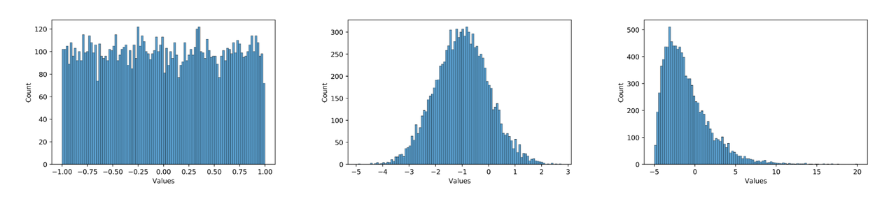
那么
尽量少
使用 精度 风险 过大 的 算子,详见 op 文档。 保证
多次 调用 的 共享 算子 每次 调用 的 输出 分布 差异 不要 太 大,或者 将 共享 算子 拆开 分别 单独 使用。 避免
多 输入 算子 不同 输入 的 数值 范围 差异 过大。 使用 int16 量化
数值 范围 和 误差 都 非常 大 的 op 。可 通过 debug 工具 找到 这 类 op 。 通过
调大 weight decay ,增加 数据 增强 等 方式 防止 模型 过 拟合。过 拟合 模型 容易 出现 较大 数值,且 对 输入 非常 敏感,轻微 的 误差 可能 导致 输出 完全 错误。 使用 BN 。
对模型
输入 做 关于0对称 的 归一化。
需要
6.4.3.2. qconfig 详解
什么是 qconfig
模型
目前,Plugin 中维护了两个版本的qconfig,早期版本的 qconfig 将在不久的将来被废弃,我们只推荐您使用此文档中介绍的 qconfig 用法。
如何获取 qconfig
使用
封装 好 的 qconfig 变量。这些 qconfig 存放 在 horizon_plugin_pytorch/quantization/qconfig.py中,可以适用 于 绝大多数 情况。包括:
from horizon_plugin_pytorch.quantization.qconfig import (
    default_calib_8bit_fake_quant_qconfig,
    default_qat_8bit_fake_quant_qconfig,
    default_qat_8bit_fixed_act_fake_quant_qconfig,
    default_calib_8bit_weight_16bit_act_fake_quant_qconfig,
    default_qat_8bit_weight_16bit_act_fake_quant_qconfig,
    default_qat_8bit_weight_16bit_fixed_act_fake_quant_qconfig,
    default_qat_8bit_weight_32bit_out_fake_quant_qconfig, # 参考算子列表,支持高精度输出的算子可以设置此 qconfig 获得更高的精度
    default_calib_8bit_weight_32bit_out_fake_quant_qconfig, # 参考算子列表,支持高精度输出的算子可以设置此 qconfig 获得更高的精度
)
使用
get_default_qconfig接口。此接口 较 固定 qconfig 变量 更 灵活,我们 推荐 您 对 量化 和 硬件 限制 有 清晰 认知 之后 再 使用。常用 参数 和 解释 如下:
from horizon_plugin_pytorch.quantization.qconfig import get_default_qconfig

qconfig = get_default_qconfig(
    activation_fake_quant="fake_quant",  # 支持 fake_quant, lsq, pact,常用 fake quant
    weight_fake_quant="fake_quant", # 支持 fake_quant, lsq, pact,常用 fake quant
    activation_observer="min_max", # 支持 min_max, fixed_scale, clip, percentile, clip_std, mse, kl
    weight_observer="min_max", # 支持 min_max, fixed_scale, clip, percentile, clip_std, mse, kl
    activation_qkwargs={
        "dtype": qint16, # 由具体算子决定是否支持 int16
        "is_sync_quantize": False, # 是否同步统计数据,默认关闭提升forward速度
        "averaging_constant": 0.01 # 滑动平均系数,设置为0时,scale不更新
    },
    weight_qkwargs={ # 只支持 dtype = qint8, qscheme = torch.per_channel_symmetric, ch_axis = 0, 不建议做额外配置
        "dtype": qint8,
        "qscheme": torch.per_channel_symmetric,
        "ch_axis": 0,
    },
)
如何设置 qconfig
共有
直接
设置 qconfig 属性。此 方法 优先级 最高,其余 方法 不会 覆盖 直接 设置 的 qconfig。
model.qconfig = default_qat_8bit_fake_quant_qconfig
qconfig 模板。在 prepare 接口
上 指定 qconfig setter 和 example_inputs,自动 为 模型 设置 qconfig。
model = prepare_qat_fx(
    model,
    example_inputs=data,
    qconfig_setter=default_qat_qconfig_setter,
)
qconfig_dict。在 prepare_qat_fx 接口
上 指定 qconfig_dict。此 用法 将 逐步 废弃,如 无 兼容性 需求,不 推荐 再 使用,这里 不 展开 介绍。
model = prepare_qat_fx(
    model,
    qconfig_dict={"": default_qat_qconfig_setter},
)
qconfig 模板
长期以来,配置 qconfig 出错
qat_model = prepare_qat_fx(
    model,
    example_inputs=example_input,  # 用来感知图结构
    qconfig_setter=( # qconfig 模板,支持传入多个模板,优先级从高到低。
        sensitive_op_qat_8bit_weight_16bit_act_qconfig_setter(table, ratio=0.2),
        default_calibration_qconfig_setter,
    )
)
模板的优先级低于直接给模型设置 qconfig 属性,如果模型在 prepare 之前已经使用 model.qconfig = xxx 进行了配置,那么模板将不会生效。如果没有特殊需求,我们不推荐将两者混合使用,这很容易引发低级错误。绝大多数情况下,我们推荐您使用模板和 model.qconfig = xxx 两种设置方式中的一种即可满足需求。
模板
固定
模板。固定 模板 中 calibration / qat / qat_fixed_act_scale 区别 在于 使用 的 observer 类型 和 scale 更新 逻辑,分别 用于 校准,qat 训练,固定 activation scale qat 训练。default 模板( default_calibration_qconfig_setter / default_qat_qconfig_setter / default_qat_fixed_act_qconfig_setter )会 做 三件 事:首先,将 可以 设置 的 高精度 输出 都 设置 上,对于 不 支持 高精度 的 输出 将 给出 提示;然后,从 grid sample 算子 的 grid 输入 向前 搜索,直到 出现 第一个 gemm 类算子 或者QuantStub,将 中间 的 所有 算子 都 设置 为 int16。根据 经验 这里 的 grid 一般 表达 范围 较 宽,int8 有 较大 可能 不 满足 精度 需求;最后,将 其余 算子 设置 为 int8。int16 模板( qat_8bit_weight_16bit_act_qconfig_setter / qat_8bit_weight_16bit_fixed_act_qconfig_setter / calibration_8bit_weight_16bit_act_qconfig_setter )会 做 两件事:首先,将 可以 设置 的 高精度 输出 都 设置 上,对于 不 支持 高精度 的 输出 将 给出 提示;其次,将 其余 算子 设置 为 int16。
from horizon_plugin_pytorch.quantization.qconfig_template import (
    default_calibration_qconfig_setter,
    default_qat_qconfig_setter,
    default_qat_fixed_act_qconfig_setter,
    qat_8bit_weight_16bit_act_qconfig_setter,
    qat_8bit_weight_16bit_fixed_act_qconfig_setter,
    calibration_8bit_weight_16bit_act_qconfig_setter,
)
敏感度
模板。敏感度 模板 有 sensitive_op_calibration_8bit_weight_16bit_act_qconfig_setter, sensitive_op_qat_8bit_weight_16bit_act_qconfig_setter, sensitive_op_qat_8bit_weight_16bit_fixed_act_qconfig_setter,三者 的 区别 和 固定 模板 中 三者 的 区别 一致,也 是 分别 用于 校准,qat 训练,固定 activation scale qat 训练。 敏感度 模板 的 第一个 输入 是 精度 debug 工具 产生 的 敏感度 结果,第二个 参数 可以 指定 ratio 或 topk ,敏感度 模板 会 将 量化 敏感度 最高 的 topk 个 算子 设置 为 int16。搭配 固定 模板,可以 轻松 实现 混合 精度 调优。
from horizon_plugin_pytorch.quantization.qconfig_template import (
    default_calibration_qconfig_setter,
    default_qat_qconfig_setter,
    default_qat_fixed_act_qconfig_setter,
    qat_8bit_weight_16bit_act_qconfig_setter,
    qat_8bit_weight_16bit_fixed_act_qconfig_setter,
    calibration_8bit_weight_16bit_act_qconfig_setter,
    sensitive_op_qat_8bit_weight_16bit_act_qconfig_setter,
    sensitive_op_qat_8bit_weight_16bit_fixed_act_qconfig_setter,
    sensitive_op_calibration_8bit_weight_16bit_act_qconfig_setter,
)

table = torch.load("output_0-0_dataindex_1_sensitive_ops.pt")

qat_model = prepare_qat_fx(
    model,
    example_inputs=example_input,
    qconfig_setter=(
        sensitive_op_qat_8bit_weight_16bit_fixed_act_qconfig_setter(table, ratio=0.2),
        default_calibration_qconfig_setter,
    )
)
自定义
模板。自定义 模板 只有 ModuleNameQconfigSetter,需要 传入 模块 名 和 对应 qconfig 的 字典,一般 用于 设置 fixed scale 等 特殊 需求,可以 和 固定 模板,敏感度 模板 搭配 使用。
from horizon_plugin_pytorch.quantization.qconfig_template import (
    default_calibration_qconfig_setter,
    default_qat_qconfig_setter,
    default_qat_fixed_act_qconfig_setter,
    qat_8bit_weight_16bit_act_qconfig_setter,
    qat_8bit_weight_16bit_fixed_act_qconfig_setter,
    calibration_8bit_weight_16bit_act_qconfig_setter,
    sensitive_op_qat_8bit_weight_16bit_act_qconfig_setter,
    sensitive_op_qat_8bit_weight_16bit_fixed_act_qconfig_setter,
    sensitive_op_calibration_8bit_weight_16bit_act_qconfig_setter,
    ModuleNameQconfigSetter,
)

table = torch.load("output_0-0_dataindex_1_sensitive_ops.pt")

module_name_to_qconfig = {
    "op_1": default_qat_8bit_fake_quant_qconfig,
    "op_2": get_default_qconfig(
        activation_observer="fixed_scale",
        activation_qkwargs={
            "dtype": qint16,
            "scale": OP2_MAX / QINT16_MAX,
        },
    )
}

qat_model = prepare_qat_fx(
    model,
    example_inputs=example_input,
    qconfig_setter=(
        ModuleNameQconfigSetter(module_name_to_qconfig),
        sensitive_op_qat_8bit_weight_16bit_fixed_act_qconfig_setter(table, ratio=0.2),
        default_calibration_qconfig_setter,
    )
)
6.4.3.3. Calibration 指南
在
流程和示例
Calibration 与 QAT 的
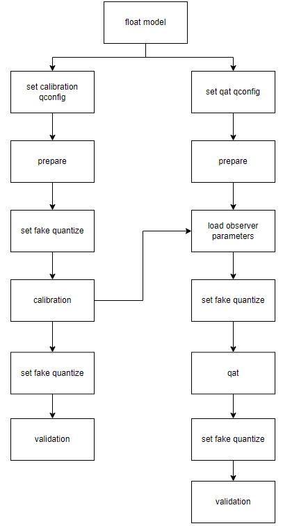
下面
构建
并 训练 浮点 模型。参考 horizon_plugin_pytorch 快速 入门 章节 中 的 获取 浮点 小节模型 内容。 在
浮点 模型 上 插入 Observer 节点。参考 horizon_plugin_pytorch 快速 入门 章节 中 的 Calibration 小节 内容。使用 prepare_qat_fx方法转化 浮点 模型 前,需要 为 模型 设置 qconfig。model.qconfig = horizon.quantization.get_default_qconfig()
get_default_qconfig可以为 weight和activation设置不同 的 observer。目前,calibration 可选 observer有 “min_max”、 “percentile”、 “mse”、 “kl” 和 “mix”。如无 特殊 需求, weight_observer推荐使用 默认 的 “min_max”, activation_observer推荐使用 “mse”。特殊 用法 和 调试 技巧 见 下面 的 常见 算法 介绍。 fake_quant参数对 Calibration 结果 无 影响,保留 默认 状态 即可。 def get_default_qconfig( activation_fake_quant: Optional[str] = "fake_quant", weight_fake_quant: Optional[str] = "fake_quant", activation_observer: Optional[str] = "min_max", weight_observer: Optional[str] = "min_max", activation_qkwargs: Optional[Dict] = None, weight_qkwargs: Optional[Dict] = None, ):
设置
fake quantize状态为 CALIBRATION。horizon.quantization.set_fake_quantize(model, horizon.quantization.FakeQuantState.CALIBRATION)
fake quantize一共有 三种 状态,分别 需要 在 QAT、calibration、validation前将 模型 的 fake quantize设置为 对应 的 状态。在 calibration 状态 下,仅 观测 各 算子 输入输出 的 统计 量。在 QAT 状态 下,除 观测 统计 量外 还 会 进行 伪 量化 操作。而 在 validation 状态 下,不会 观测 统计 量,仅 进行 伪 量化 操作。 class FakeQuantState(Enum): QAT = "qat" CALIBRATION = "calibration" VALIDATION = "validation"
calibration。把
准备 好 的 校准 数据 喂给 模型,模型 在 forward 过程 中 由 observer 观测 相关 统计 量。 设置
模型 状态 为 eval 并 设置 fake quantize状态为 VALIDATION。model.eval() horizon.quantization.set_fake_quantize(model, horizon.quantization.FakeQuantState.VALIDATION)
验证
calibration效果。如果效果 满意,则 可以 直接 将 模型 转为 定点 或 在 此基础 上 进行 量化 训练,不 满意 则 调整 calibration qconfig中的 参数 继续 calibration。
常用算法介绍
备注:
有关每个算子的参数说明,请参考文末 API 文档。
| 算法 | 速度 |
精度 |
易用性 |
|---|---|---|---|
| min_max | 1 | 5 | 1 |
| percentile | 2 | 4 | 4 |
| mse | 4 | 1 | 2 |
| kl | 5 | 2 | 3 |
| mix | 3 | 2 | 1 |
常用
对于
min_max。此
方法 仅 统计 最大值 最小值 的 滑动 平均,用于 快速 确定 Batch size、average_constant 等 通用 参数,没有 太 多 技巧。 percentile。此
方法 是 所有 方法 中 精度 上限 最高 的,但 也 是 调整 起来 最 麻烦 的,如果 通过 其他 方法 或本 方法 的 默认 参数 就 可以 满足 精度 要求,那么 不 建议 在 调 参 上 花太多 时间。percentile 可调 的 参数 一共 有 两个 bins、percentile。bins 越 多,max 的 候选 项 间隔 越小,可 供 调整 的 粒度 越细,但 也 意味着 更 高 的 计算 耗时。建议 先 确定 percentile 再 调整 bins,两者 交替 迭代 缩小 调参 范围 直至 达到 满意 的 效果。绝大部分 情况 下 bins 取 2048 提供 的 调整 粒度 完全 足够,不 需要 单独 调整 这个 参数。以下 是 一个 模型 的 调参 路径:
| 顺序 | percentile | bins | 精度 |
|---|---|---|---|
| 1 | 99.99 | 2048 | 53.75 |
| 2 | 99.99 | 4096 | 54.38 |
| 3 | 99.995 | 4096 | 16.25 |
| 4 | 99.985 | 4096 | 32.67 |
| 5 | 99.9875 | 4096 | 57.06 |
| 6 | 99.9875 | 8192 | 62.84 |
| 7 | 99.98875 | 8192 | 57.62 |
| 8 | 99.988125 | 8192 | 63.15 |
在
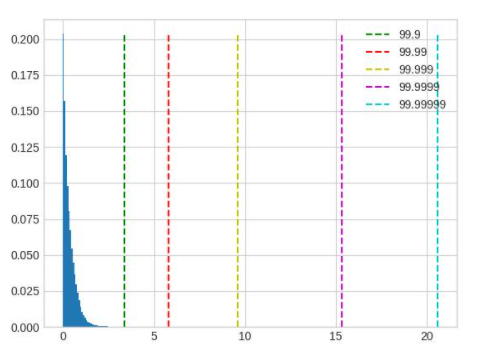
超
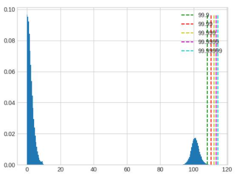
值域
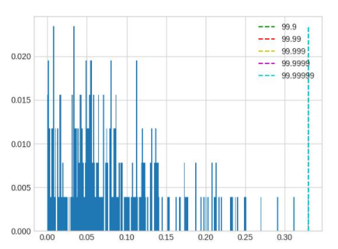
layernorm 的
mse。可
调整 的 参数 只有 stride,默认 stride 为 1,会 逐步 尝试 最大值 的 100 分位 并 选出 量化 反 量化 前后 误差 最小(L2 距离)的 分位 对应 的 值。此 方法 对大 模型 耗时 较 高,在 合理 范围 内 调 大 stride 可以 在 保证 精度 的 前提 下 减少 耗时,stride 调整 过 大会 影响 精度。注意,调整 此 方法 的 参数 只能 优化 耗时,并 不能 显著 提升 精度。 kl。可调
的 参数 一共 有 两个 bin 和 update_interval。由于 此 方法 耗时 过长,不 建议 调整 默认 bin。update_interval 默认 为 1,表示 间隔 多少 个 forward step 计算 一次 KL,调大 可以 减少 耗时(不 影响 精度),但 需要 保证 update_interval 不 超过 总 的 calibration step,否则 无法 得到 正常 的 量化 参数。一般 推荐 ,这样直接 将 update_interval 设 为 calibration step 前面 的 forward step 只 采集 数据 更新 直方图,只有 最后 一个 step 才 会 计算 KL 和 scale,可以 最大 程度 减少 KL 的 耗时,同时 由于 最终 的 直方图 包含 所有 输入 数据 的 统计 信息,因此 不会 对 精度 造成 影响。 mix。此
方法 为 混合 校准,对于 每 一个 需要 统计 的 地方,都 会 尝试 percentile 方法 的 不同 参数,选出 量化 反 量化 前后 误差 最小(L2 距离)的 方法。自动化 程度较高,没有 需要 调整 的 参数。
调参技巧
calibration 数据
越多越好,但 因为 边际效应 的 存在,当 数据量 大到 一定 程度 后,对 精度 的 提升 将 非常 有限。如果 训练 集较 小,可以 全部 用来 calibration,如果 训练 集 较大,可以 结合 calibration 耗时 挑选 大小 合适 的 子集,建议 至少 进行 10 - 100 个 step 的 校准。 数据
可以 做 水平 翻转 这 类 augmentation,不要 做 马赛克 这种 augmentation。尽量 使用 infer 阶段 的 前 处理 + 训练 数据 进行 校准。 Batch size 尽可能
大,如果 数据 噪声 较大 或 模型 离群 点较 多,可以 适当 减小。此参数 应当 在 尝试 min max 方法 时 确定。 average_constant 表示
每个 step 对 最大值 最小值 的 影响,average_constant 越小,当前 step 的 影响 越小,历史 滑动 均值 的 影响 越大。该 参数 需要 结合 数据量 在 0.01 ~ 0.5 之间 调整。当 数据量 充足 时(step > 100),average_constant 取 0.01,数据量 不足 时,average_constant 酌情 增加,极端 情况 下,只有 2 个 step 的 数据,average_constant 取 0.5。此参数 应当 在 尝试 min max 方法 时 确定,之后 其他 方法 都 沿用 此参数。 calibration 模型
精度 较 好 时,固定 feature map 的 量化 参数 进行 QAT 训练 可以 取得 更好 的 效果,精度 较差 时,则 不能 固定 calibration 得到 的 量化 参数。关于 精度 是 好 还是 坏,没有 明确 的 标准,需要 去 尝试。比如:某 模型 精度 为 100,如果 calibration 精度 为 50,那么 精度 肯定 称不上 好,但 如果 calibration 精度 为 95,那么 这个 精度 是否 可以 达到 固定 feature map 量化 参数 的 程度 就 需要 尝试 了,通常 做法 是 固定 与 不 固定 都 做 实验 进行 对比。 优先
尝试 min max 方法,该 方法 是 速度 最快 的,用来 跑通 calibration 流程,调整 并 确定 batch size 和 average_constant 两个 参数,接着 分别 尝试 percentile、kl、mse 和 mix 四种 方法 并 选取 效果 最好 的 方法。
Observer 参数文档
class horizon_plugin_pytorch.quantization.observer_v2.KLObserver(
    bins: int = 512,
    update_interval: int = 1,
    averaging_constant: float = 0.01,
    ch_axis: int = -1,
    dtype: Union[torch.dtype, horizon_plugin_pytorch.dtype.QuantDType] = 'qint8',
    qscheme: torch.qscheme = torch.per_tensor_symmetric,
    quant_min: int = None,
    quant_max: int = None,
    is_sync_quantize: bool = False,
    factory_kwargs: Dict = None
)
KL 观察器(KLObserver)
基于
参数:
bins – Number of histograms bins.
update_interval – Interval of computing KL entropy and update min/max. KLObserver will constantly collect histograms of activations, but only perform KL calculation when update_interval is satisfied. if it is set to 1, KL entropy will be computed every forward step. Larger interval guarantees less time and does no harm to calibration accuracy. Set it to the total calibration steps can achieve best performance. update_interval must be no greater than total calibration steps, otherwise no min/max will be computed.
averaging_constant – Averaging constant for min/max.
ch_axis – Channel axis.
dtype – Quantized data type.
qscheme – Quantization scheme to be used.
quant_min – Min quantization value. Will follow dtype if unspecified.
quant_max – Max quantization value. Will follow dtype if unspecified.
is_sync_quantize – If sync statistics when training with multiple devices.
factory_kwargs – kwargs which are passed to factory functions for min_val and max_val.
forward(x_orig)
定义
所有
提示:
尽管
class horizon_plugin_pytorch.quantization.observer_v2.MSEObserver(
    stride: int = 1,
    averaging_constant: float = 0.01,
    ch_axis: int = -1,
    dtype: Union[torch.dtype, horizon_plugin_pytorch.dtype.QuantDType] = 'qint8',
    qscheme: torch.qscheme = torch.per_tensor_symmetric,
    quant_min: int = None,
    quant_max: int = None,
    is_sync_quantize: bool = False,
    factory_kwargs: Dict = None
)
MSE 观察器(MSEObserver)
用于
该
参数:
stride – 搜索
步长。值越 大,搜索 空间 越小,计算 时间 越短,但 精度 可能 下降。默认值 为 1,建议 不 超过 20。 averaging_constant – 用于 min/max 的
平滑 系数。 ch_axis – 通道
轴。 dtype – 量化
后 的 数据类型。 qscheme – 使用
的 量化 方案。 quant_min – 最小
量化 值。未指定 时 根据 dtype 自动 推断。 quant_max – 最大
量化 值。未指定 时 根据 dtype 自动 推断。 is_sync_quantize – 是否
在 使用 多 设备 训练 时 同步 统计 信息。 factory_kwargs – 传递
给 min_val 和 max_val 工厂 函数 的 关键字 参数。
forward(x_orig)
定义
所有
提示:
尽管
class horizon_plugin_pytorch.quantization.observer_v2.MinMaxObserver(
    averaging_constant: float = 0.01,
    ch_axis: int = -1,
    dtype: Union[torch.dtype, horizon_plugin_pytorch.dtype.QuantDType] = 'qint8',
    qscheme: torch.qscheme = torch.per_tensor_symmetric,
    quant_min: int = None,
    quant_max: int = None,
    is_sync_quantize: bool = False,
    factory_kwargs: Dict = None
)
MinMax 观察器(MinMaxObserver)
该
参数:
averaging_constant – 用于 min/max 的
平滑 系数。 ch_axis – 通道
轴。 dtype – 量化
后 的 数据类型。 qscheme – 使用
的 量化 方案。 quant_min – 最小
量化 值。未指定 时 根据 dtype 自动 推断。 quant_max – 最大
量化 值。未指定 时 根据 dtype 自动 推断。 is_sync_quantize – 是否
在 使用 多 设备 训练 时 同步 统计 信息。 factory_kwargs – 传递
给 min_val 和 max_val 工厂 函数 的 关键字 参数。
forward(x_orig)
记录 x 的
class horizon_plugin_pytorch.quantization.observer_v2.MixObserver(
    averaging_constant: float = 0.01,
    ch_axis: int = -1,
    dtype: Union[torch.dtype, horizon_plugin_pytorch.dtype.QuantDType] = 'qint8',
    qscheme: torch.qscheme = torch.per_tensor_symmetric,
    quant_min: int = None,
    quant_max: int = None,
    is_sync_quantize: bool = False,
    factory_kwargs: Dict = None
)
Mix 观察器(MixObserver)
该
参数:
averaging_constant – 用于 min/max 的
平滑 系数。 ch_axis – 通道
轴。 dtype – 量化
后 的 数据类型。 qscheme – 使用
的 量化 方案。 quant_min – 最小
量化 值。未指定 时 根据 dtype 自动 推断。 quant_max – 最大
量化 值。未指定 时 根据 dtype 自动 推断。 is_sync_quantize – 是否
在 使用 多 设备 训练 时 同步 统计 信息。 factory_kwargs – 传递
给 min_val 和 max_val 工厂 函数 的 关键字 参数。
forward(x_orig)
定义
所有
提示:
尽管
class horizon_plugin_pytorch.quantization.observer_v2.PercentileObserver(
    percentile: float = 99.99,
    bins: int = 2048,
    averaging_constant: float = 0.01,
    ch_axis: int = -1,
    dtype: Union[torch.dtype, horizon_plugin_pytorch.dtype.QuantDType] = 'qint8',
    qscheme: torch.qscheme = torch.per_tensor_symmetric,
    quant_min: int = None,
    quant_max: int = None,
    is_sync_quantize: bool = False,
    factory_kwargs: Dict = None
)
百分位
基于
参数:
percentile – 直方图
的 百分位 索引。 bins – 直方图
的 分桶 数。 averaging_constant – 用于 min/max 的
平滑 系数。 ch_axis – 通道
轴。 dtype – 量化
后 的 数据类型。 qscheme – 使用
的 量化 方案。 quant_min – 最小
量化 值。未指定 时 根据 dtype 自动 推断。 quant_max – 最大
量化 值。未指定 时 根据 dtype 自动 推断。 is_sync_quantize – 是否
在 使用 多 设备 训练 时 同步 统计 信息。 factory_kwargs – 传递
给 min_val 和 max_val 工厂 函数 的 关键字 参数。
forward(x_orig)
定义
所有
提示:
尽管
class horizon_plugin_pytorch.quantization.MovingAverageMinMaxObserver(
    averaging_constant=0.01,
    dtype=torch.qint8,
    qscheme=torch.per_tensor_symmetric,
    quant_min=None,
    quant_max=None,
    is_sync_quantize=False,
    factory_kwargs=None
)
滑动
用于
该
参数:
averaging_constant – 用于 min/max 的
平滑 系数。 dtype – 量化
后 的 数据类型。 qscheme – 使用
的 量化 方案,仅 支持 per_tensor_symmetric。 reduce_range – 将
量化 数据类型 的 范围 减少 1 位。 quant_min – 最小
量化 值。 quant_max – 最大
量化 值。 is_sync_quantize – 是否
使用 同步 量化。 factory_kwargs – 用于
注册 数据 缓冲区 的 参数。
forward(x_orig)
记录 x 的
class horizon_plugin_pytorch.quantization.MovingAveragePerChannelMinMaxObserver(
    averaging_constant=0.01,
    ch_axis=0,
    dtype=torch.qint8,
    qscheme=torch.per_channel_symmetric,
    quant_min=None,
    quant_max=None,
    is_sync_quantize=False,
    factory_kwargs=None
)
滑动
用于
该
参数:
averaging_constant – 用于 min/max 的
平滑 系数。 ch_axis – 通道
轴。 dtype – 量化
后 的 数据类型。 qscheme – 使用
的 量化 方案,仅 支持 per_channel_symmetric。 quant_min – 最小
量化 值。 quant_max – 最大
量化 值。 is_sync_quantize – 是否
使用 同步 量化。 factory_kwargs – 用于
注册 数据 缓冲区 的 参数。
forward(x_orig)
定义
所有
提示:
尽管
6.4.3.4. 量化感知训练指南
量化
量化
流程和示例
虽然
from horizon_plugin_pytorch.quantization import get_default_qconfig
# 将模型转为 QAT 状态
default_qat_8bit_fake_quant_qconfig = get_default_qconfig(
    activation_fake_quant="fake_quant",
    weight_fake_quant="fake_quant",
    activation_observer="min_max",
    weight_observer="min_max",
    activation_qkwargs=None,
    weight_qkwargs={
        "qscheme": torch.per_channel_symmetric,
        "ch_axis": 0,
    },
)
default_qat_out_8bit_fake_quant_qconfig = get_default_qconfig(
    activation_fake_quant=None,
    weight_fake_quant="fake_quant",
    activation_observer=None,
    weight_observer="min_max",
    activation_qkwargs=None,
    weight_qkwargs={
        "qscheme": torch.per_channel_symmetric,
        "ch_axis": 0,
    },
)
qat_model = prepare_qat_fx(
    float_model,
    {
        "": default_qat_8bit_fake_quant_qconfig,
        "module_name": {
            "classifier": default_qat_out_8bit_fake_quant_qconfig,
        },
    },
).to(device)
# 加载 Calibration 模型中的量化参数
qat_model.load_state_dict(calib_model.state_dict())
# 进行量化感知训练
# 作为一个 filetune 过程,量化感知训练一般需要设定较小的学习率
optimizer = torch.optim.SGD(
    qat_model.parameters(), lr=0.0001, weight_decay=2e-4
)

for nepoch in range(epoch_num):
    # 注意此处对 QAT 模型 training 状态的控制方法
    qat_model.train()
    set_fake_quantize(qat_model, FakeQuantState.QAT)

    train_one_epoch(
        qat_model,
        nn.CrossEntropyLoss(),
        optimizer,
        None,
        train_data_loader,
        device,
    )

    # 注意此处对 QAT 模型 eval 状态的控制方法
    qat_model.eval()
    set_fake_quantize(qat_model, FakeQuantState.VALIDATION)

    # 测试 qat 模型精度
    top1, top5 = evaluate(
        qat_model,
        eval_data_loader,
        device,
    )
    print(
        "QAT model: evaluation Acc@1 {:.3f} Acc@5 {:.3f}".format(
            top1.avg, top5.avg
        )
    )

# 测试 quantized 模型精度
quantized_model = convert_fx(qat_model.eval()).to(device)

top1, top5 = evaluate(
    quantized_model,
    eval_data_loader,
    device,
)
print(
    "Quantized model: evaluation Acc@1 {:.3f} Acc@5 {:.3f}".format(
        top1.avg, top5.avg
    )
)
注意:
由于
由
prepare_qat_fx
加载 Calibration 模型
参数
prepare_qat_fx
这一
加载 Calibration 模型参数
通过
训练迭代
至此,完成
伪量化算子
量化
备注:
由于 BPU 只
伪量化过程
以 int8 量化
fake_quant_x = clip(round(x / scale),-128, 127) * scale
和 Conv2d 通过
基于统计的方法
量化
def compute_scale(x: Tensor):
    xmin, xmax = x.max(), maxv = x.min()
    return max(xmin.abs(), xmax.abs()) / 256.0
由于 Tensor 中MovingAverageMinMaxObserver 等。
在default_qat_8bit_fake_quant_qconfig 及其
基于学习的方法
虽然 round 的
def round_ste(x: Tensor):
    return (x.round() - x).detach() + x
在default_qat_8bit_lsq_quant_qconfig 及其
有
6.4.3.5. 异构模型指南
异构模型介绍
异构
包含 BPU 不
支持 算子 的 模型。 由于
量化 精度 误差 过大,用户 指定 某些 算子 运行 在 CPU 上 的 模型。
使用流程

通过 prepare 将
备注:
用户
算子限制
由于
主要接口参数说明
horizon_plugin_pytorch.quantization.prepare_qat_fx
设置
hybrid=True来开启 异构 模型 功能。 用户
可以 通过 设置 hybrid_dict参数来 强制 指定 某些 BPU 支持 的 算子 跑 在 CPU 上。
def prepare_qat_fx(
    model: Union[torch.nn.Module, GraphModule],
    qconfig_dict: Dict[str, Any] = None,
    prepare_custom_config_dict: Dict[str, Any] = None,
    optimize_graph: bool = False,
    hybrid: bool = False,
    hybrid_dict: Dict[str, List] = None,
) -> ObservedGraphModule:
    """Prepare QAT 模型
        `model`: torch.nn.Module 或 GraphModule(使用 fuse_fx 后的模型)
        `qconfig_dict`: 定义 Qconfig。如果除了 qconfig_dict 以外,还使用了 eager mode 在 module 内定义 qconfig 的方式,则 module 内定义的 qconfig 优先生效。qconfig_dict 的配置格式如下:
            qconfig_dict = {
                # 可选,全局配置
                "": qconfig,
                # 可选,按 module 类型配置
                "module_type": [(torch.nn.Conv2d, qconfig), ...],
                # 可选,按 module 名配置
                "module_name": [("foo.bar", qconfig),...],
                # 优先级:global < module_type < module_name < module.qconfig
                # 非 module 类型的算子的 qconfig 默认与其父 module 的 qconfig 保持一致,如果需要单独设置,请将这部分单独封装成 module。
            }
        `prepare_custom_config_dict`: 自定义配置字典
            prepare_custom_config_dict = {
                # 暂时只支持 preserved_attributes。一般而言会自动保留所有属性,这个选项只是以防万一,几乎不会用到。
                "preserved_attributes": ["preserved_attr"],
            }
        `optimize_graph`: 保持 cat 输入输出 scale 一致,目前只有在 Bernoulli 架构下有效。
        `hybrid`: 是否使用异构模式。在以下情况下必须打开异构模式:
            1. 模型包含 BPU 不支持的算子或用户希望指定部分 BPU 算子退回 CPU。
            2. 用户希望 QAT 模型与 horizon_nn 对接进行定点化。
        `hybrid_dict`: 定义用户主动指定的 CPU 算子。
            hybrid_dict = {
                # 可选,按 module 类型配置
                "module_type": [torch.nn.Conv2d, ...],
                # 可选,按 module 名配置
                "module_name": ["foo.bar", ...],
                # 优先级:module_type < module_name
                # 与 qconfig_dict 类似,如果想要非 module 类型的算子运行在 CPU 上,需要将这部分单独封装成 module。
            }
    """
horizon_plugin_pytorch.utils.onnx_helper.export_to_onnx
导出 onnx 模型,从而hb_mapper 。
备注:
该
def export_to_onnx(
    model,
    args,
    f,
    export_params=True,
    verbose=False,
    training=TrainingMode.EVAL,
    input_names=None,
    output_names=None,
    operator_export_type=OperatorExportTypes.ONNX_FALLTHROUGH,
    opset_version=11,
    do_constant_folding=True,
    example_outputs=None,
    strip_doc_string=True,
    dynamic_axes=None,
    keep_initializers_as_inputs=None,
    custom_opsets=None,
    enable_onnx_checker=False,
):
    """此接口与 torch.onnx.export 基本一致,隐藏了无需修改的参数,需要的注意参数有:
        `model`: 需要 export 的模型
        `args`: 模型输入,用于 trace 模型
        `f`: 保存的 onnx 文件名或文件描述符
        `operator_export_type`: 算子导出类型
            1. 对于非异构模型,onnx 仅用于可视化,不需要保证实际可用,使用默认值 OperatorExportTypes.ONNX_FALLTHROUGH
            2. 对于异构模型,onnx 需要保证实际可用,使用 None 确保导出的为标准 onnx 算子。
        `opset_version`: 只能为 11,horizon_plugin_pytorch 在 opset 11 中注册了特定的映射规则。
        注意:如果使用公版 torch.onnx.export,需要确保上述参数设置正确,
        并且 import horizon_plugin_pytorch.utils._register_onnx_ops
        以向 opset 11 中注册特定的映射规则。
    """
horizon_plugin_pytorch.quantization.convert_fx
异构convert_fx 把
注意:
通过 convert_fx 得到
def convert_fx(
    graph_module: GraphModule,
    convert_custom_config_dict: Dict[str, Any] = None,
    _remove_qconfig: bool = True,
) -> QuantizedGraphModule:
    """转换 QAT 模型,仅用于评测定点模型。
        `graph_module`: 经过 prepare->(calibration)->train 之后的模型
        `convert_custom_config_dict`: 自定义配置字典
            convert_custom_config_dict = {
                # 暂时只支持 preserved_attributes。一般而言会自动保留所有属性,这个选项只是以防万一,几乎不会用到。
                "preserved_attributes": ["preserved_attr"],
            }
        `_remove_qconfig`: convert 之后是否删除 qconfig,一般不会用到
    """
流程和示例
改造
浮点 模型。 插入
QuantStub与DeQuantStub,保持与非 异构 的 用法 一致。 如果
第一个 op 是 cpu op,那么不 需要 插入 QuantStub。如果
最后 一个 op 是 cpu op,那么可以 不用 插入 DeQuantStub。
对于
非 module的运算,如果 需要 单独 设置 qconfig或指定 其 运行 在 CPU 上,需要 将 其 封装 成 module,参考示例 中 的 _SeluModule。
设置
march。 X3 设置bernoulli2, X5 设置为bayes-e。 设置
qconfig。保留非 异构 模式 下 在 module内设置 qconfig的配置 方式,除此以外,还 可以 通过 prepare_qat_fx接口的 qconfig_dict参数传入 qconfig,具体用法 见 接口 参数 说明。 对于
BPU op,必须保证 有 qconfig,如果其 输入 op 不 为 QuantStub,那么还 需要 保证 该 输入 op 有 activation qconfig。对于
CPU op,qconfig不会对 其 产生 任何 影响,但 如果 后面 接 BPU op,则必须 有 qconfig。推荐
设置 方式:先 设置 全局 qconfig为horizon.quantization.default_qat_8bit_fake_quant_qconfig(或者horizon.quantization.default_calib_8bit_fake_quant_qconfig,根据 calibration 或 qat 阶段选择) ,在 此基础 上 根据 需求 修改,一般而言,只 需要 对 int16 和 高精度 输出 的 op 单独 设置 qconfig。
注意:
目前BAYES_E 的 X5 支持int16 量化。
设置
hybrid_dict。可选,具体 用法 见 接口 参数 说明,如果 没有 主动 指定 的 CPU 算子,可以 不 设置 hybrid_dict。调用
prepare_qat_fx并进行 calibration。参考 horizon_plugin_pytorch 开发指南 章节 中 的 Calibration 小节 内容。 调用
prepare_qat_fx,加载calibration模型并 进行 QAT 训练。参考 horizon_plugin_pytorch 开发 指南 章节 中 的 量化 训练 小节内容。 调用
convert_fx。可选,没有 评测 定点 模型 精度 的 需求 时 可以 跳过。 调用
export_to_onnx。也可以 使用 torch.onnx.export但需要 遵守 export_to_onnx接口说明 中 的 注意事项。 使用
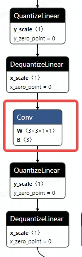
hb_mapper转换 onnx 模型。转换后 需 检查 算子 是否 运行 在 预期 的 设备 上,在 部分 情况 下, hb_mapper仍然需要 设置 run_on_cpu参数。比如:虽然conv在 QAT 阶段没有 量化,但 由于 其 输入(上 一个 算子 输出)经过 了 伪 量化, hb_mapper仍然会 默认 将 其 量化。
import copy
import numpy as np
import torch
from horizon_plugin_pytorch.march import March, set_march
from horizon_plugin_pytorch.nn import qat
from horizon_plugin_pytorch.quantization import (
    prepare_qat_fx,
    convert_fx,
    set_fake_quantize,
    FakeQuantState,
    load_observer_params,
)
from horizon_plugin_pytorch.quantization.qconfig import (
    default_calib_8bit_fake_quant_qconfig,
    default_calib_out_8bit_fake_quant_qconfig,
    default_qat_8bit_fake_quant_qconfig,
    default_qat_out_8bit_fake_quant_qconfig,
)
from torch import nn
from torch.quantization import DeQuantStub, QuantStub
from horizon_plugin_pytorch.utils.onnx_helper import export_to_onnx

class _ConvBlock(nn.Module):
    def __init__(self, channels=3):
        super().__init__()
        self.conv = nn.Conv2d(channels, channels, 1)
        self.prelu = torch.nn.PReLU()

    def forward(self, input):
        x = self.conv(input)
        x = self.prelu(x)
        return torch.nn.functional.selu(x)

# 封装 functional selu 为 module,便于单独设置
class _SeluModule(nn.Module):
    def forward(self, input):
        return torch.nn.functional.selu(input)

class HybridModel(nn.Module):
    def __init__(self, channels=3):
        super().__init__()
        # 插入 QuantStub
        self.quant = QuantStub()
        self.conv0 = nn.Conv2d(channels, channels, 1)
        self.prelu = torch.nn.PReLU()
        self.conv1 = _ConvBlock(channels)
        self.conv2 = nn.Conv2d(channels, channels, 1)
        self.conv3 = nn.Conv2d(channels, channels, 1)
        self.conv4 = nn.Conv2d(channels, channels, 1)
        self.selu = _SeluModule()
        # 插入 DequantStub
        self.dequant = DeQuantStub()
        self.identity = torch.nn.Identity()

    def forward(self, input):
        x = self.quant(input)
        x = self.conv0(x)
        x = self.identity(x)
        x = self.prelu(x)
        x = torch.nn.functional.selu(x)
        x = self.conv1(x)
        x = self.conv2(x)
        x = self.conv3(x)
        x = self.identity(x)
        x = self.conv4(x)
        x = self.selu(x)
        return self.dequant(x)

# 设置 march **X3** 设置BERNOULLI2, **X5** 设置为BAYES_E。
set_march(March.XXX)
data_shape = [1, 3, 224, 224]
data = torch.rand(size=data_shape)
model = HybridModel()
qat_model = copy.deepcopy(model)
# float 模型的推理不要放在 prepare_qat_fx 之后,prepare_qat_fx 会对 float 模型做 inplace 修改
float_res = model(data)

calibration_model = prepare_qat_fx(
    model,
    {
        "": default_calib_8bit_fake_quant_qconfig,
        # selu 为 cpu 算子,conv4 实际上是 bpu 模型的输出,设置为高精度输出
        "module_name": [("conv4", default_calib_out_8bit_fake_quant_qconfig)]
    },
    hybrid=True,
    hybrid_dict={
        "module_name": ["conv1.conv", "conv3"],
        "module_type": [_SeluModule],
    },
)
# calibration 阶段需确保原有模型不会发生变化
calibration_model.eval()
set_fake_quantize(calibration_model, FakeQuantState.CALIBRATION)

for i in range(5):
    calibration_model(torch.rand(size=data_shape))

qat_model = prepare_qat_fx(
    qat_model,
    {
        "": default_qat_8bit_fake_quant_qconfig,
        # selu 为 cpu 算子,conv4 实际上是 bpu 模型的输出,设置为高精度输出
        "module_name": [("conv4", default_qat_out_8bit_fake_quant_qconfig)]
    },
    hybrid=True,
    hybrid_dict={
        "module_name": ["conv1.conv", "conv3"],
        "module_type": [_SeluModule],
    },
)

load_observer_params(calibration_model, qat_model)
set_fake_quantize(calibration_model, FakeQuantState.QAT)

# qat training start
# ......
# qat training end

# 导出 qat.onnx
export_to_onnx(
    qat_model,
    data,
    "qat.onnx",
    operator_export_type=None,
)

# 评测定点模型
quantize_model = convert_fx(qat_model)
quantize_res = quantize_model(data)
打印 QAT 模型
HybridModel(
  (quant): QuantStub(
    (activation_post_process): FakeQuantize(
      fake_quant_enabled=tensor([1], dtype=torch.uint8), observer_enabled=tensor([1], dtype=torch.uint8),            quant_min=-128, quant_max=127, dtype=qint8, qscheme=torch.per_tensor_symmetric, ch_axis=-1,         scale=tensor([0.0078]), zero_point=tensor([0])
      (activation_post_process): MovingAverageMinMaxObserver(min_val=tensor([-0.9995]), max_val=tensor([0.9995]))
    )
  )
  (conv0): Conv2d(
    3, 3, kernel_size=(1, 1), stride=(1, 1)
    (weight_fake_quant): FakeQuantize(
      fake_quant_enabled=tensor([1], dtype=torch.uint8), observer_enabled=tensor([1], dtype=torch.uint8),            quant_min=-128, quant_max=127, dtype=qint8, qscheme=torch.per_channel_symmetric, ch_axis=0,         scale=tensor([0.0038, 0.0041, 0.0016]), zero_point=tensor([0, 0, 0])
      (activation_post_process): MovingAveragePerChannelMinMaxObserver(min_val=tensor([-0.4881, -0.4944,  0.0787]), max_val=tensor([-0.1213,  0.5284,  0.1981]))
    )
    (activation_post_process): FakeQuantize(
      fake_quant_enabled=tensor([1], dtype=torch.uint8), observer_enabled=tensor([1], dtype=torch.uint8),            quant_min=-128, quant_max=127, dtype=qint8, qscheme=torch.per_tensor_symmetric, ch_axis=-1,         scale=tensor([0.0064]), zero_point=tensor([0])
      (activation_post_process): MovingAverageMinMaxObserver(min_val=tensor([-0.8159]), max_val=tensor([0.8159]))
    )
  )
  (prelu): PReLU(num_parameters=1)
  (conv1): _ConvBlock(
    (conv): Conv2d(3, 3, kernel_size=(1, 1), stride=(1, 1))
    (prelu): PReLU(num_parameters=1)
  )
  (conv2): Conv2d(
    3, 3, kernel_size=(1, 1), stride=(1, 1)
    (weight_fake_quant): FakeQuantize(
      fake_quant_enabled=tensor([1], dtype=torch.uint8), observer_enabled=tensor([1], dtype=torch.uint8),            quant_min=-128, quant_max=127, dtype=qint8, qscheme=torch.per_channel_symmetric, ch_axis=0,         scale=tensor([0.0040, 0.0044, 0.0040]), zero_point=tensor([0, 0, 0])
      (activation_post_process): MovingAveragePerChannelMinMaxObserver(min_val=tensor([-0.5044, -0.4553, -0.5157]), max_val=tensor([0.1172, 0.5595, 0.4104]))
    )
    (activation_post_process): FakeQuantize(
      fake_quant_enabled=tensor([1], dtype=torch.uint8), observer_enabled=tensor([1], dtype=torch.uint8),            quant_min=-128, quant_max=127, dtype=qint8, qscheme=torch.per_tensor_symmetric, ch_axis=-1,         scale=tensor([0.0059]), zero_point=tensor([0])
      (activation_post_process): MovingAverageMinMaxObserver(min_val=tensor([-0.7511]), max_val=tensor([0.7511]))
    )
  )
  (conv3): Conv2d(3, 3, kernel_size=(1, 1), stride=(1, 1))
  (conv4): Conv2d(
    3, 3, kernel_size=(1, 1), stride=(1, 1)
    (weight_fake_quant): FakeQuantize(
      fake_quant_enabled=tensor([1], dtype=torch.uint8), observer_enabled=tensor([1], dtype=torch.uint8),            quant_min=-128, quant_max=127, dtype=qint8, qscheme=torch.per_channel_symmetric, ch_axis=0,         scale=tensor([0.0025, 0.0037, 0.0029]), zero_point=tensor([0, 0, 0])
      (activation_post_process): MovingAveragePerChannelMinMaxObserver(min_val=tensor([-0.2484, -0.4718, -0.3689]), max_val=tensor([ 0.3239, -0.0056,  0.3312]))
    )
    (activation_post_process): None
  )
  (selu): _SeluModule()
  (dequant): DeQuantStub()
  (identity): Identity()
  (prelu_input_dequant): DeQuantStub()
  (selu_1_activation_post_process): _WrappedCalibFakeQuantize(
    (activation_post_process): FakeQuantize(
      fake_quant_enabled=tensor([1], dtype=torch.uint8), observer_enabled=tensor([1], dtype=torch.uint8),            quant_min=-128, quant_max=127, dtype=qint8, qscheme=torch.per_tensor_symmetric, ch_axis=-1,         scale=tensor([0.0042]), zero_point=tensor([0])
      (activation_post_process): MovingAverageMinMaxObserver(min_val=tensor([-0.5301]), max_val=tensor([0.5301]))
    )
  )
  (conv3_activation_post_process): _WrappedCalibFakeQuantize(
    (activation_post_process): FakeQuantize(
      fake_quant_enabled=tensor([1], dtype=torch.uint8), observer_enabled=tensor([1], dtype=torch.uint8),            quant_min=-128, quant_max=127, dtype=qint8, qscheme=torch.per_tensor_symmetric, ch_axis=-1,         scale=tensor([0.0072]), zero_point=tensor([0])
      (activation_post_process): MovingAverageMinMaxObserver(min_val=tensor([-0.9156]), max_val=tensor([0.9156]))
    )
  )
  (conv3_input_dequant): DeQuantStub()
  (selu_2_input_dequant): DeQuantStub()
)

def forward(self, input):
    input_1 = input
    quant = self.quant(input_1);  input_1 = None
    conv0 = self.conv0(quant);  quant = None
    identity = self.identity(conv0);  conv0 = None
    prelu_input_dequant_0 = self.prelu_input_dequant(identity);  identity = None
    prelu = self.prelu(prelu_input_dequant_0);  prelu_input_dequant_0 = None
    selu = torch.nn.functional.selu(prelu, inplace = False);  prelu = None
    conv1_conv = self.conv1.conv(selu);  selu = None
    conv1_prelu = self.conv1.prelu(conv1_conv);  conv1_conv = None
    selu_1 = torch.nn.functional.selu(conv1_prelu, inplace = False);  conv1_prelu = None
    selu_1_activation_post_process = self.selu_1_activation_post_process(selu_1);  selu_1 = None
    conv2 = self.conv2(selu_1_activation_post_process);  selu_1_activation_post_process = None
    conv3_input_dequant_0 = self.conv3_input_dequant(conv2);  conv2 = None
    conv3 = self.conv3(conv3_input_dequant_0);  conv3_input_dequant_0 = None
    conv3_activation_post_process = self.conv3_activation_post_process(conv3);  conv3 = None
    identity_1 = self.identity(conv3_activation_post_process);  conv3_activation_post_process = None
    conv4 = self.conv4(identity_1);  identity_1 = None
    selu_2_input_dequant_0 = self.selu_2_input_dequant(conv4);  conv4 = None
    selu_2 = torch.nn.functional.selu(selu_2_input_dequant_0, inplace = False);  selu_2_input_dequant_0 = None
    dequant = self.dequant(selu_2);  selu_2 = None
    return dequant
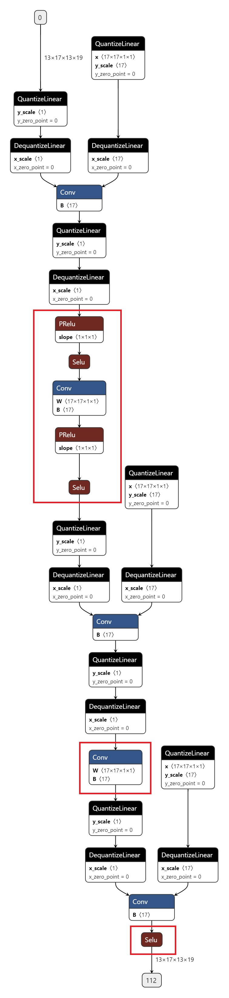
导出
6.4.3.6. 精度调优工具使用指南
由于
原有
浮点 模型 不利于 量化,如 存在 共享 op 或 共享 结构; QAT 网络结构
或 配置 异常,如 模型 中 存在 没有 fuse 的 pattern,没有 设置 高精度 输出 等; 某些
算子 对 量化 比较 敏感,该 算子 的 量化 误差 在 前 向 传播 过程 中 逐层 累积,最终 导致 模型 输出 误差 较大。
针对
模型
结构 :检查检查 模型 中 是否 存在 共享 op、没有 fuse 的 pattern 或者 不 符合 预期 的 量化 配置; QuantAnalysis:自动
比 对 分析 两个 模型,定位 到 量化 模型 中 异常 算子 或者 量化 敏感 op; ModelProfiler:获得
模型 中 每 一个 op 的 数值 特征 信息,如 输入输出 的 最大 最小值 等。
快速上手
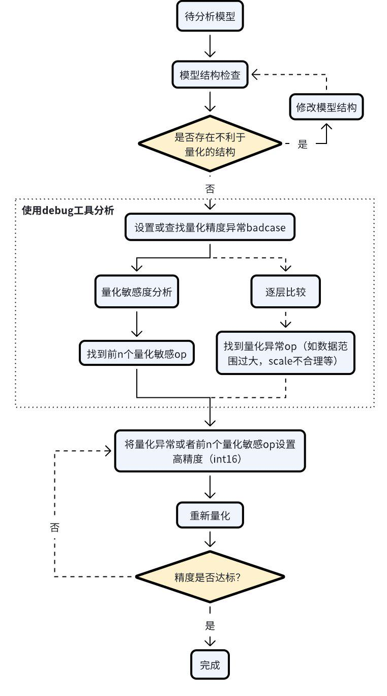
当
检查
模型 中 是否 存在 不利于 量化 的 结构 或者 异常 配置; 使用 QuantAnalysis 模块
进行 分析,具体步骤 如下: 找到
一个 bad case 作为 模型 的 输入。bad case 是 指 基准 模型 和 待 分析模型 输出 相差 最大 的 那个 输入; 进行
量化 敏感度 分析,目前 的 经验 是 L1 敏感度 排序 前 n 个 通常 为 量化 敏感 op(不同 的 模型 n 的 数值 不 一样,暂无 自动 确定 的 方法,需要 手动 尝试,如 前 10 个,20 个…)。将 量化 敏感 op 设置 高精度 量化(如 int16 量化),重新 进行 量化 流程; 或者
逐层 比较 两个 模型 的 输入输出 等 信息,检查 是否 存在 数据 范围 过大 或者 scale 不合理 等 量化 异常 的 op,如 某些 具有 物理 含义 的 op 应 设置 固定 scale。
整体
一个
    from copy import deepcopy

    import torch
    from torch import nn
    from torch.quantization import DeQuantStub, QuantStub

    from horizon_plugin_pytorch.march import March, set_march
    from horizon_plugin_pytorch.quantization.qconfig import (
        default_qat_8bit_fake_quant_qconfig,
    )
    from horizon_plugin_pytorch.quantization.quantize_fx import prepare_qat_fx
    from horizon_plugin_pytorch.quantization import hbdk4 as hb4
    from horizon_plugin_pytorch.utils.check_model import check_qat_model
    from horizon_plugin_profiler import QuantAnalysis, ModelProfiler


    class Net(nn.Module):
        def __init__(self):
            super(Net, self).__init__()
            self.conv = nn.Conv2d(3, 3, 1)
            self.relu = nn.ReLU()
            self.quant = QuantStub()
            self.dequant = DeQuantStub()

        def forward(self, x):
            x = self.quant(x)
            x = self.conv(x)
            x = self.relu(x)
            x = torch.nn.functional.interpolate(
                x, scale_factor=1.3, mode="bilinear", align_corners=False
            )
            x = self.dequant(x)
            return x

    data = torch.rand((1, 3, 32, 32))
    float_net = Net()
    float_net(data)

    set_march(March.XXX)
    float_net.qconfig = default_qat_8bit_fake_quant_qconfig

    qat_net = deepcopy(float_net)
    qat_net = prepare_qat_fx(qat_net)

    ############################### 模型结构检查 ##############################
    # 确认提示的异常层是否符合预期
    check_qat_model(qat_net, data, save_results=True)
    ##########################################################################

    qat_net(data)

    quantized_net = deepcopy(qat_net)
    quantized_net = convert_fx(quantized_net)

    ############################### quant analysis ############################

    # 1. 初始化
    qa = QuantAnalysis(
        baseline_model=float_net,
        analysis_model=qat_net,
        analysis_model_type="fake_quant",
        out_dir="./floatvsqat",
    )

    # 也支持对比 qat 和 quantized
    # qa = QuantAnalysis(
    #     baseline_model=qat_net,
    #     analysis_model=quantized_net,
    #     analysis_model_type="quantized",
    #     out_dir="./qatvsquantized",
    # )

    # 2. 设置 badcase 输入。
    qa.set_bad_case(data)

    # 实际场景下推荐使用 auto_find_bad_case 在整个 dataloader 上搜索 bad case
    # 也支持设置 num_steps 参数来控制搜索的范围
    # qa.auto_find_bad_case(your_dataloader, num_steps=100)

    # 3. 运行两个模型
    qa.run()

    # 4. 两个模型逐层比较。确认 abnormal_layer_advisor.txt 提示的异常层是否符合预期
    # qa.compare_per_layer()

    # 5. 计算敏感度节点。可以将 topk 排序的敏感度节点设置高精度来尝试提升量化模型精度
    qa.sensitivity()

    ##########################################################################
API Reference
模型结构检查
    # from horizon_plugin_pytorch.utils.check_model import check_qat_model

    def check_qat_model(
        model: torch.nn.Module,
        example_inputs: Any,
        save_results: bool = False,
        out_dir: Optional[str] = None,
    ):
检查 calibration/qat 模型
参数
model: 待
检查 模型 example_inputs: 模型
输入 save_results: 是否
将 检查 结果 保存 到 txt 文件。默认 False。 out_dir: 结果
文件 ‘model_check_result.txt’ 的 保存 路径。默认 空,保存 到 当前 路径 下。
输出
屏幕
输出:检查 出 的 异常 层 model_check_result.txt:在 save_results = True 时
生成。主要 由5部分 组成 未 fuse 的 pattern
每个 module 的
调用 次数。正常 每个 op 仅 调用 1 次,0 表示 未 被 调用,超过 1 次则 表示 被 共享 了 多次; 每个 op 输出
的 qconfig 配置; 每个 op weight(如果
有 的话)的 qconfig 配置; 异常 qconfig 提示(如果
有 的话)。
Fusable modules are listed below:
name    type
------  -----------------------------------------------------
conv    <class 'horizon_plugin_pytorch.nn.qat.conv2d.Conv2d'>
relu    <class 'horizon_plugin_pytorch.nn.qat.relu.ReLU'>


Each module called times:
name       called times
-------  --------------
conv                  1
relu                  1
quant                 1
dequant               1

Each layer out qconfig:
+---------------+-----------------------------------------------------------+---------------+---------------+----------------+-----------------------------+
| Module Name   | Module Type                                               | Input dtype   | out dtype     | ch_axis        | observer                    |
|---------------+-----------------------------------------------------------+---------------+---------------+----------------+-----------------------------|
| quant         | <class 'horizon_plugin_pytorch.nn.qat.stubs.QuantStub'>   | torch.float32 | qint8         | -1             | MovingAverageMinMaxObserver |
| conv          | <class 'horizon_plugin_pytorch.nn.qat.conv2d.Conv2d'>     | qint8         | qint8         | -1             | MovingAverageMinMaxObserver |
| relu          | <class 'horizon_plugin_pytorch.nn.qat.relu.ReLU'>         | qint8         | qint8         | qconfig = None |                             |
| dequant       | <class 'horizon_plugin_pytorch.nn.qat.stubs.DeQuantStub'> | qint8         | torch.float32 | qconfig = None |                             |
+---------------+-----------------------------------------------------------+---------------+---------------+----------------+-----------------------------+

Weight qconfig:
+---------------+-------------------------------------------------------+----------------+-----------+---------------------------------------+
| Module Name   | Module Type                                           | weight dtype   |   ch_axis | observer                              |
|---------------+-------------------------------------------------------+----------------+-----------+---------------------------------------|
| conv          | <class 'horizon_plugin_pytorch.nn.qat.conv2d.Conv2d'> | qint8          |         0 | MovingAveragePerChannelMinMaxObserver |
+---------------+-------------------------------------------------------+----------------+-----------+---------------------------------------+
`prepare_qat/prepare_qat_fx` 流程中也已集成该接口,您可以设置 `verbose=1` 打开该检查功能。我们推荐您在进行 QAT 训练之前,使用此接口进行检查,并根据检查结果对模型做针对性的调整。
QuantAnalysis 类
QuantAnalysis 类
class QuantAnalysis(object):
    def __init__(
        self,
        baseline_model: torch.nn.Module,
        analysis_model: torch.nn.Module,
        analysis_model_type: str,
        out_dir: Optional[str] = None,
    )
参数
baseline_model: 基准
模型(高精度) analysis_model:待
分析 的 模型(精度 掉 点) analysis_model_type: 待
分析 的 模型 类型。支持 两种 输入 fake_quant:待
分析 的 模型 可以 是 精度 掉 点 的 calibration/qat 模型,此时 基准 模型 可以 是 原始 浮点 模型 或者 一个 精度 达标 的 int8/int16 混合 配置 的 calibration/qat 模型 quantized:待
分析 的 模型 是 精度 掉 点 的 定点 问题,此时 基准 模型 必须 是 一个 精度 达标 的 calibration/qat 模型
out_dir:指定
比较 结果 的 输出 目录
该类
auto_find_bad_case
    def auto_find_bad_case(
        self,
        data_generator: Iterable,
        num_steps: Optional[int] = None,
        metric: str = "L1",
        device: Optional[Union[torch.device, str, int]] = None,
        custom_metric_func: Optional[Callable] = None,
        custom_metric_order_seq: Optional[str] = None,
    ):
自动
参数
data_generator:dataloader 或者
一个 自定义 的 迭代 器,每次 迭代 产生 一个 数据 num_steps:迭代 steps 次数
metric:指定
何种 metric 作为 badcase 的 metric。默认 使用 L1 最差 的 结果。支持 Cosine/MSE/L1/KL/SQNR/custom。若 为 custom,表示 使用 自定义 的 metric 计算方法,此时 custom_metric_func 和 custom_metric_order_seq 两个 参数 必须 不 为 None device:指定
模型 运行 device custom_metric_func:自定义
模型 输出 比较 函数 custom_metric_order_seq:自定义
模型 输出 比较 函数 的 排序 规则,仅 支持 “ascending”/”descending”,表示 升序/降序
set_bad_case
def set_bad_case(self, data)
手动
参数
data: badcase输入
load_bad_case
def load_bad_case(self, filename: Optional[str] = None)
从
参数
filename:指定
的 文件 路径
save_bad_case
def save_bad_case(self)
将 badcase 保存
set_model_profiler_dir
    def set_model_profiler_dir(
        self,
        baseline_model_profiler_path: str,
        analysis_model_profiler_path: str,
    ):
手动
某些
参数
baseline_model_profiler_path:基准
模型 的 profiler 路径 analysis_model_profiler_path:待
分析模型 的 profiler 路径
run
    def run(
        self,
        device: Optional[Union[torch.device, str, int]] = None,
    )
运行
参数
device:模型
运行 的 device
compare_per_layer
def compare_per_layer(self)
比较
输出
abnormal_layer_advisor.txt: 所有
异常 层,包括 相似 度低/数据 范围 过大/输入 没有 归一化/输出 没有 高精度 等 情况 profiler.html: 可视化
展示 所有 metric 指标 及 模型 中 每 一层 的 数据 范围 diff
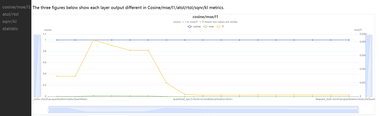
compare_per_layer_out.txt: 以
表格 的 形式 展示 模型 中 每层 layer 的 具体 信息,包括 各种 指标、数据 范围、量化 dtype 等。从左到右 每 一列 分别 表示: Index:op index
mod_name:该 op 名字,若 op 为 module 类型,则
显示 该 module 在 模型 中 的 prefix name,若 为 function 类型,则 不 显示 base_op_type:基准
模型 中该 op 的 type,可能 是 module 类型 或者 function 名称 analy_op_type:待
分析模型 中该 op 的 type,可能 是 module 类型 或者 function 名称 Shape:该 op 输出
的 shape quant_dtype:该 op 输出
的 量化 类型 Qscale:该 op 输出
的 量化 scale Cosine:该 op 在
两个 模型 中 输出 的 余弦 相似 度 MSE:该 op 在
两个 模型 中 输出 的 MSE 距离 L1:该 op 在
两个 模型 中 输出 的 L1 距离 KL:该 op 在
两个 模型 中 输出 的 KL 相似 度 SQNR:该 op 在
两个 模型 中 输出 的 SQNR 相似 度 Atol:该 op 在
两个 模型 中 输出 的 绝对误差 Rtol:该 op 在
两个 模型 中 输出 的 相对误差 base_model_min:基准
模型 中该 op 输出 的 最小值 analy_model_min:待
分析模型 中该 op 输出 的 最小值 base_model_max:基准
模型 中该 op 输出 的 最大值 analy_model_max:待
分析模型 中该 op 输出 的 最大值 base_model_mean:基准
模型 中该 op 输出 的 平均值 analy_model_mean:待
分析模型 中该 op 输出 的 平均值 base_model_var:基准
模型 中该 op 输出 的 方差 analy_model_var:待
分析模型 中该 op 输出 的 方差
+----+------------+--------------------------------------------------------------------+--------------------------------------------------------------------+----------------------------+---------------+-----------+-----------+-----------+-----------+-----------+------------+-----------+-------------------------------------------------+------------------+-------------------+------------------+-------------------+-------------------+--------------------+------------------+-------------------+
|    | mod_name   | base_op_type                                                       | analy_op_type                                                      | shape                      | quant_dtype   |    qscale |    Cosine |       MSE |        L1 |        KL |       SQNR |      Atol |                                            Rtol |   base_model_min |   analy_model_min |   base_model_max |   analy_model_max |   base_model_mean |   analy_model_mean |   base_model_var |   analy_model_var |
|----+------------+--------------------------------------------------------------------+--------------------------------------------------------------------+----------------------------+---------------+-----------+-----------+-----------+-----------+-----------+------------+-----------+-------------------------------------------------+------------------+-------------------+------------------+-------------------+-------------------+--------------------+------------------+-------------------|
|  0 | quant      | torch.ao.quantization.stubs.QuantStub                              | horizon_plugin_pytorch.nn.qat.stubs.QuantStub                      | torch.Size([1, 3, 32, 32]) | qint8         | 0.0078354 | 0.9999924 | 0.0000052 | 0.0019757 | 0.0000006 | 48.1179886 | 0.0039178 |                                       1.0000000 |        0.0003164 |         0.0000000 |        0.9990171 |         0.9950994 |         0.5015678 |          0.5014852 |        0.0846284 |         0.0846521 |
|  1 | conv       | torch.nn.modules.conv.Conv2d                                       | horizon_plugin_pytorch.nn.qat.conv2d.Conv2d                        | torch.Size([1, 3, 32, 32]) | qint8         | 0.0060428 | 0.9999037 | 0.0000085 | 0.0023614 | 0.0000012 | 37.1519432 | 0.0096008 |                                      48.2379990 |       -0.7708085 |        -0.7674332 |        0.4674263 |         0.4652941 |        -0.0411330 |         -0.0412943 |        0.0423415 |         0.0422743 |
|  2 | relu       | torch.nn.modules.activation.ReLU                                   | horizon_plugin_pytorch.nn.qat.relu.ReLU                            | torch.Size([1, 3, 32, 32]) | qint8         | 0.0060428 | 0.9998640 | 0.0000037 | 0.0010231 | 0.0000004 | 35.5429153 | 0.0093980 |                                      48.2379990 |        0.0000000 |         0.0000000 |        0.4674263 |         0.4652941 |         0.0641222 |          0.0639115 |        0.0090316 |         0.0089839 |
|  3 |            | horizon_plugin_pytorch.nn.interpolate.autocasted_interpolate_outer | horizon_plugin_pytorch.nn.interpolate.autocasted_interpolate_outer | torch.Size([1, 3, 41, 41]) | qint8         | 0.0060428 | 0.9234583 | 0.0012933 | 0.0245362 | 0.0001882 |  8.1621437 | 0.1928777 | 340282346638528859811704183484516925440.0000000 |        0.0000000 |         0.0000000 |        0.3509629 |         0.3504813 |         0.0643483 |          0.0639483 |        0.0043305 |         0.0043366 |
|  4 | dequant    | torch.ao.quantization.stubs.DeQuantStub                            | horizon_plugin_pytorch.nn.qat.stubs.DeQuantStub                    | torch.Size([1, 3, 41, 41]) | torch.float32 |           | 0.9234583 | 0.0012933 | 0.0245362 | 0.0001882 |  8.1621437 | 0.1928777 | 340282346638528859811704183484516925440.0000000 |        0.0000000 |         0.0000000 |        0.3509629 |         0.3504813 |         0.0643483 |          0.0639483 |        0.0043305 |         0.0043366 |
+----+------------+--------------------------------------------------------------------+--------------------------------------------------------------------+----------------------------+---------------+-----------+-----------+-----------+-----------+-----------+------------+-----------+-------------------------------------------------+------------------+-------------------+------------------+-------------------+-------------------+--------------------+------------------+-------------------+
compare_per_layer_out.csv: 以 csv 的
格式 展示 每层 的 具体 信息。内容 和 compare_per_layer_out.txt 完全一致,csv 文件 的 存储 格式 方便 您 通过 excel 等 软件 打开 分析。
sensitivity
    def sensitivity(
        self,
        device: Optional[torch.device] = None,
        metric: str = "L1",
        reserve: bool = False
    ):
模型
sensitivity 函数不支持计算 hbir 模型的敏感度。
参数
device:指定
模型 运行 的 device metric:相似
度 排序 的 metric,默认 L1,支持 Cosine/MSE/L1/KL/SQNR reserve:是否
反序 打印 敏感度 节点,以 支持 将 某些 int16 算子 退回 int8 来 提升 上板 性能
输出
sensitive_ops.txt。文件
中 按照 量化 敏感度 从 高到 低 的 顺序排列 op。从左到右 每 一列 分别 表示: op_name:op 名字,
sensitive_type:计算
量化 敏感 的 类型,包括 三种 activation:仅
量化 该 op 输出 的 量化 敏感度 weight:仅
量化 该 op 权重 的 量化 敏感度 both:同时
量化 该 op 输出 和 权重 的 量化 敏感度
op_type:op 类型
metric:计算
敏感度 的 指标。按照 敏感度 从 高到 低 的 顺序 排序。支持 Cosine/L1/MSE/KL/SQNR 五种 指标。默认 使用 L1。 L1:取值
范围 [0, $+\infty$],数值 越大则 该 op 对 量化 越 敏感(从大到 小 排序) Cosine:取值
范围 [0,1],越 接近 0 则 该 op 对 量化 越 敏感(从小到大 排序) MSE:取值
范围 [0, $+\infty$],数值 越大则 该 op 对 量化 越 敏感(从大到 小 排序) KL:取值
范围 [0, $+\infty$],数值 越大则 该 op 对 量化 越 敏感(从大到 小 排序) SQNR:取值
范围 [0, $+\infty$],数值 越小则 该 op 对 量化 越 敏感(从小到大 排序)
sensitive_ops.pt。使用 torch.save 保存
的 敏感度 排序 的 列表,方便 您 后续 加载 使用。列表 格式 见返回值部分 说明。
返回值
敏感度 List,List 中[op_name, sensitive_type, op_type, metric1, metric2, ...]。
整个 List 示例
[
    [op1, "activation", op1_type, L1],
    [op2, "activation", op2_type, L1],
    [op3, "activation", op3_type, L1],
    [op1, "weight", op1_type, L1],
    [op2, "both", op2_type, L1],
    ...
]
您
op_name    sensitive_type    op_type                                                         L1
---------  ----------------  -------------------------------------------------------  ---------
quant      activation        <class 'horizon_plugin_pytorch.nn.qat.stubs.QuantStub'>  0.0245567
conv       activation        <class 'horizon_plugin_pytorch.nn.qat.conv2d.Conv2d'>    0.0245275
conv       both              <class 'horizon_plugin_pytorch.nn.qat.conv2d.Conv2d'>    0.0245275
conv       weight            <class 'horizon_plugin_pytorch.nn.qat.conv2d.Conv2d'>    0.024501
clean
def clean(self)
清除
ModelProfiler 类
统计
# from horizon_plugin_profiler import ModelProfiler

class ModelProfiler(object):
    def __init__(
        self,
        model: torch.nn.Module,
        out_dir: str,
    )
参数
model: 需要
统计 的 模型 out_dir: 相关
文件 保存 的 路径
该类仅支持通过 with 语句的方式使用。
with ModelProfiler(net, "./profiler_dir") as p:
    net(data)

p.get_info_manager.table()
p.get_info_manager.tensorboard()
该类
get_info_manager
def get_info_manager(self)
获得
返回值
管理OpRunningInfoManager。其中
table
class OpRunningInfoManager:
    def table(
        self,
        out_dir: str = None,
        prefixes: Tuple[str, ...] = None,
        types: Tuple[Type, ...] = None,
        with_stack: bool = False,
    )
在
参数
out_dir:statistic.txt 文件
的 存储 路径,默认 None,存储 到 self.out_dir prefixes:需要
统计 的 模型 中 op 的 prefixes 。默认 统计 所有 op types:需要
统计 的 模型 中 op 的 type。默认 统计 所有 op with_stack: 是否
显示 每个 op 在 代码 中 对应 的 位置
输出
statistic.txt 文件,从左到右
Index: op index
Op Name:op type,module 类名
或者 function 名 Mod Name:若
是 module 类,则 显示 该 module 在 模型 中 的 prefix name;若 是 function 类型,则 显示 该 function 所在 的 module prefix name。 Attr:input/output/weight/bias
Dtype:tensor 的
数据类型 Scale:tensor 的 scale
Min:当前 tensor 的
最小值 Max:当前 tensor 的
最大值 Mean:当前 tensor 的
平均值 Var:当前 tensor 中
数值 的 方差 Shape:tensor shape
+---------+--------------------------------------------------------------------+------------+--------+---------------+-----------+------------+-----------+------------+-----------+----------------------------+
| Index   | Op Name                                                            | Mod Name   | Attr   | Dtype         | Scale     | Min        | Max       | Mean       | Var       | Shape                      |
|---------+--------------------------------------------------------------------+------------+--------+---------------+-----------+------------+-----------+------------+-----------+----------------------------|
| 0       | horizon_plugin_pytorch.nn.qat.stubs.QuantStub                      | quant      | input  | torch.float32 |           | 0.0003164  | 0.9990171 | 0.5015678  | 0.0846284 | torch.Size([1, 3, 32, 32]) |
| 0       | horizon_plugin_pytorch.nn.qat.stubs.QuantStub                      | quant      | output | qint8         | 0.0078354 | 0.0000000  | 0.9950994 | 0.5014852  | 0.0846521 | torch.Size([1, 3, 32, 32]) |
| 1       | horizon_plugin_pytorch.nn.qat.conv2d.Conv2d                        | conv       | input  | qint8         | 0.0078354 | 0.0000000  | 0.9950994 | 0.5014852  | 0.0846521 | torch.Size([1, 3, 32, 32]) |
| 1       | horizon_plugin_pytorch.nn.qat.conv2d.Conv2d                        | conv       | weight | torch.float32 |           | -0.5315086 | 0.5750652 | 0.0269936  | 0.1615299 | torch.Size([3, 3, 1, 1])   |
| 1       | horizon_plugin_pytorch.nn.qat.conv2d.Conv2d                        | conv       | bias   | torch.float32 |           | -0.4963555 | 0.4448483 | -0.0851902 | 0.2320642 | torch.Size([3])            |
| 1       | horizon_plugin_pytorch.nn.qat.conv2d.Conv2d                        | conv       | output | qint8         | 0.0060428 | -0.7674332 | 0.4652941 | -0.0412943 | 0.0422743 | torch.Size([1, 3, 32, 32]) |
| 2       | horizon_plugin_pytorch.nn.qat.relu.ReLU                            | relu       | input  | qint8         | 0.0060428 | -0.7674332 | 0.4652941 | -0.0412943 | 0.0422743 | torch.Size([1, 3, 32, 32]) |
| 2       | horizon_plugin_pytorch.nn.qat.relu.ReLU                            | relu       | output | qint8         | 0.0060428 | 0.0000000  | 0.4652941 | 0.0639115  | 0.0089839 | torch.Size([1, 3, 32, 32]) |
| 3       | horizon_plugin_pytorch.nn.interpolate.autocasted_interpolate_outer |            | input  | qint8         | 0.0060428 | 0.0000000  | 0.4652941 | 0.0639115  | 0.0089839 | torch.Size([1, 3, 32, 32]) |
| 3       | horizon_plugin_pytorch.nn.interpolate.autocasted_interpolate_outer |            | output | qint8         | 0.0060428 | 0.0000000  | 0.3504813 | 0.0639483  | 0.0043366 | torch.Size([1, 3, 41, 41]) |
| 4       | horizon_plugin_pytorch.nn.qat.stubs.DeQuantStub                    | dequant    | input  | qint8         | 0.0060428 | 0.0000000  | 0.3504813 | 0.0639483  | 0.0043366 | torch.Size([1, 3, 41, 41]) |
| 4       | horizon_plugin_pytorch.nn.qat.stubs.DeQuantStub                    | dequant    | output | torch.float32 |           | 0.0000000  | 0.3504813 | 0.0639483  | 0.0043366 | torch.Size([1, 3, 41, 41]) |
+---------+--------------------------------------------------------------------+------------+--------+---------------+-----------+------------+-----------+------------+-----------+----------------------------+
tensorboard
class OpRunningInfoManager:
    def tensorboard(
        self,
        out_dir: str = None,
        prefixes: Tuple[str, ...] = None,
        types: Tuple[Type, ...] = None,
        force_per_channel: bool = False,
    ):
在 tensorboard 中
参数
out_dir: tensorboard 相关
文件 保 目录。默认 保存 到 self.out_dir/tensorboard 目录 下 prefixes:需要
统计 的 模型 中 op 的 prefixes。默认 统计 所有 types:需要
统计 的 模型 中 op 的 type。默认 统计 所有 force_per_channel:是否
以 per_channel 量化 的 方式 展示 直方图
输出
tensorboard 文件,打开
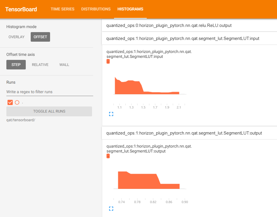
6.4.3.7. 量化部署 PT 模型的跨设备 Inference 说明
量化
若to(device) 操作
下面
import torch


class Net(torch.nn.Module):
    def forward(self, x: torch.Tensor):
        y = torch.ones(x.shape, device=x.device)
        z = torch.zeros_like(x)

        return y + z


script_mod = torch.jit.trace(
    Net(), torch.rand(2, 3, 3, 3, device=torch.device("cpu"))
)
script_mod.to(torch.device("cuda"))
print(script_mod.graph)

# graph(%self : __torch__.Net,
#       %x : Float(2, 3, 3, 3, strides=[27, 9, 3, 1], requires_grad=0, device=cpu)):
#   %4 : int = prim::Constant[value=0]()
#   %5 : int = aten::size(%x, %4)
#   %6 : Long(device=cpu) = prim::NumToTensor(%5)
#   %16 : int = aten::Int(%6)
#   %7 : int = prim::Constant[value=1]()
#   %8 : int = aten::size(%x, %7)
#   %9 : Long(device=cpu) = prim::NumToTensor(%8)
#   %17 : int = aten::Int(%9)
#   %10 : int = prim::Constant[value=2]()
#   %11 : int = aten::size(%x, %10)
#   %12 : Long(device=cpu) = prim::NumToTensor(%11)
#   %18 : int = aten::Int(%12)
#   %13 : int = prim::Constant[value=3]()
#   %14 : int = aten::size(%x, %13)
#   %15 : Long(device=cpu) = prim::NumToTensor(%14)
#   %19 : int = aten::Int(%15)
#   %20 : int[] = prim::ListConstruct(%16, %17, %18, %19)
#   %21 : NoneType = prim::Constant()
#   %22 : NoneType = prim::Constant()
#   %23 : Device = prim::Constant[value="cpu"]()
#   %24 : bool = prim::Constant[value=0]()
#   %y : Float(2, 3, 3, 3, strides=[27, 9, 3, 1], requires_grad=0, device=cpu) = aten::ones(%20, %21, %22, %23, %24)
#   %26 : int = prim::Constant[value=6]()
#   %27 : int = prim::Constant[value=0]()
#   %28 : Device = prim::Constant[value="cpu"]()
#   %29 : bool = prim::Constant[value=0]()
#   %30 : NoneType = prim::Constant()
#   %z : Float(2, 3, 3, 3, strides=[27, 9, 3, 1], requires_grad=0, device=cpu) = aten::zeros_like(%x, %26, %27, %28, %29, %30)
#   %32 : int = prim::Constant[value=1]()
#   %33 : Float(2, 3, 3, 3, strides=[27, 9, 3, 1], requires_grad=0, device=cpu) = aten::add(%y, %z, %32)
#   return (%33)
可以to(torch.device("cuda")) 后,模型aten::ones 和 aten::zeros_like 的 device 参数prim::Constant[value="cpu"](),因此to(device) 只能ScriptModule 的 graph。
torch 官方
针对
PT 模型执行使用的 device 和 trace 不一致
对于cuda:0,即torch.cuda.set_device 接口,将cuda:0 trace 出
若 trace 时horizon_plugin_pytorch.jit.to_device 接口
from horizon_plugin_pytorch.jit import to_device

script_mod = to_device(script_mod, torch.device("cuda"))
print(script_mod.graph)

# graph(%self : __torch__.Net,
#       %x.1 : Tensor):
#   %38 : bool = prim::Constant[value=0]()
#   %60 : Device = prim::Constant[value="cuda"]()
#   %34 : NoneType = prim::Constant()
#   %3 : int = prim::Constant[value=0]()
#   %10 : int = prim::Constant[value=1]()
#   %17 : int = prim::Constant[value=2]()
#   %24 : int = prim::Constant[value=3]()
#   %41 : int = prim::Constant[value=6]()
#   %4 : int = aten::size(%x.1, %3)
#   %5 : Tensor = prim::NumToTensor(%4)
#   %8 : int = aten::Int(%5)
#   %11 : int = aten::size(%x.1, %10)
#   %12 : Tensor = prim::NumToTensor(%11)
#   %15 : int = aten::Int(%12)
#   %18 : int = aten::size(%x.1, %17)
#   %19 : Tensor = prim::NumToTensor(%18)
#   %22 : int = aten::Int(%19)
#   %25 : int = aten::size(%x.1, %24)
#   %26 : Tensor = prim::NumToTensor(%25)
#   %32 : int = aten::Int(%26)
#   %33 : int[] = prim::ListConstruct(%8, %15, %22, %32)
#   %y.1 : Tensor = aten::ones(%33, %34, %34, %60, %38)
#   %z.1 : Tensor = aten::zeros_like(%x.1, %41, %3, %60, %38, %34)
#   %50 : Tensor = aten::add(%y.1, %z.1, %10)
#   return (%50)
多卡并行推理
在to_device 的cuda:0 上torch.cuda.set_device 的
import os
import torch
import signal
import torch.distributed as dist
import torch.multiprocessing as mp
from horizon_plugin_pytorch.jit import to_device

model_path = "path_to_pt_model_file"

def main_func(rank, world_size, device_ids):
    torch.cuda.set_device(device_ids[rank])
    dist.init_process_group("nccl", rank=rank, world_size=world_size)

    model = to_device(torch.jit.load(model_path), torch.device("cuda"))

    # 数据加载,模型 forward,精度计算等内容此处省略

def launch(device_ids):
    try:
        world_size = len(device_ids)
        mp.spawn(
            main_func,
            args=(world_size, device_ids),
            nprocs=world_size,
            join=True,
        )
    # 当按下 Ctrl+c 时,关闭所有子进程
    except KeyboardInterrupt:
        os.killpg(os.getpgid(os.getpid()), signal.SIGKILL)

launch([0, 1, 2, 3])
上述torch.nn.parallel.DistributedDataParallel 的
6.4.3.8. 常见问题
import 出错
错误Cannot find the extension library(_C.so)
解决
确定 horizon_plugin_pytorch 版本
和 cuda 版本 是 对应 的 在 python3 中,找到 horizon_plugin_pytorch 的
执行 路径,检测 该 目录 下 是否 有 .so 文件。可能 同时 存在 多个 horizon_plugin_pytorch 的 版本,需要 卸载 只 保留 一个 需要 的 版本。
错误RuntimeError: Cannot load custom ops. Please rebuild the horizon_plugin_pytorch
解决
无法正常 prepare_calibration/qat
RuntimeError: Only Tensors created explicitly by the user (graph leaves) support the deepcopy protocol at the moment
解决
将 prepare_calibration/qat 的 inplace 设
为 True 正常 horizon_plugin_pytorch 定义
的 算子 不会 出现 这种 错误,检查 模型 中 自定义 的 算子 是否 有 non-leaf tensor 的 定义。
prepare_qat 后 forward 报错
TypeError: when calling function <built-in method conv2d of type object at >
解决
编译报错
ValueError 'unsupported node', aten::unbind
解决iter,该
量化精度异常
QAT/Quantized 精度
解决
使用 torch.jit.load 加载 pt 文件报错
RuntimeError: Unknown builtin op: horizon::bpu_scale_quantization
解决torch.jit.load 前import horizon_plugin_pytorch。否则,加载horizon.jit.save 在horizon.jit.load 会
6.4.3.9. 常见使用误区
设置类错误
warning 错误:
无需
正确
warning 错误:
没有
正确
## X5 需要使用 Bayes-e
horizon.march.set_march(horizon.march.March.Bayes)

## X3 需要使用 Bernoulli2
horizon.march.set_march(horizon.march.March.Bernoulli2)
warning 错误:
模型
错误
class ToyNet(nn.Module):
    def __init__(self):
        self.conv0 = nn.Conv2d(4,4,3,3)
        self.relu0 = nn.ReLU()
        self.classifier = nn.Conv2d(4,4,3,3)

    def forward(self, x):
        out = self.conv0(x)
        out = self.relu(out)
        out = self.classifier(out)
        return out

# 错误的设置 qconfig 示例:

float_model = ToyNet()

qat_model = prepare_qat_fx(
    float_model,
    {
        "": default_qat_8bit_fake_quant_qconfig, # 整网设置成 int8 量化
    },
)
正确
qat_model = prepare_qat_fx(
    float_model,
    {
        "module_name": {
            "classifier": default_qat_out_8bit_fake_quant_qconfig, # 网络输出 classifier 层设置为高精度
        },
        "": default_qat_8bit_fake_quant_qconfig, # 其它层设置成 int8 量化
    },
)
方法类错误
warning 错误:
Calibration 过程
由于
warning 错误:
模型
正确
warning 错误:
量化
正确
quantized_model = convert_fx(qat_model.eval())
acc = evaluate(quantized_model, eval_data_loader, device)
网络类错误
warning 错误:
多次FloatFunctional() 定义
错误
class ToyNet(nn.Module):
    def __init__(self):
        self.add = FloatFunctional()

    def forward(self, x, y, z)
        out = self.add(x, y)
        return self.add(out, z)
正确FloatFunctional() 定义
class ToyNet(nn.Module):
    def __init__(self):
        self.add0 = FloatFunctional()
        self.add1 = FloatFunctional()

    def forward(self, x, y, z)
        out = self.add0.add(x, y)
        return self.add1.add(out, z)
算子类错误
warning 错误:
Quantized 模型
正确
模型类错误
warning 错误:
浮点
模型
对
输入 数据 稍加 变换 之后,输出 结果 变化 较大 模型
参数 赋值 较大 模型 activation 较大
正确