6.3.2. PTQ Principle and Step-by-Step Guide

6.3.2.1. Introduction

Model conversion refers to the process of transforming an original floating-point model into an X5 mixed heterogeneous model. The original floating-point model (also referred to as a floating-point model in some parts of this document) is a usable model trained using deep learning frameworks such as TensorFlow or PyTorch, with computations performed in float32 precision. A mixed heterogeneous model is a format suitable for execution on X5 processors.

This chapter will repeatedly refer to these two types of models. To avoid ambiguity, please ensure you understand this concept before proceeding.

The complete development workflow using the X5 algorithm toolchain involves five key stages: Floating-Point Model Preparation, Model Verification, Model Conversion, Performance Evaluation, and Accuracy Evaluation, as illustrated below:

model_conversion_flowchart

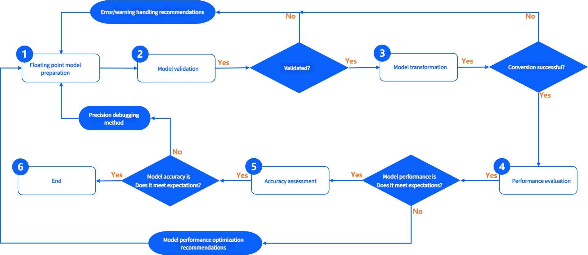
Floating-Point Model Preparation: This stage ensures the original floating-point model is in a format supported by the X5 algorithm toolchain’s model conversion tool. The floating-point model originates from models trained using DL frameworks such as TensorFlow or PyTorch. For detailed requirements and recommendations, please refer to the Floating-Point Model Preparation section.

Model Verification: This stage verifies whether the original floating-point model meets the requirements of the X5 algorithm toolchain. The X5 algorithm toolchain provides the hb_mapper checker tool for checking the floating-point model. For specific usage instructions, please refer to the Verify Model section.

Model Conversion: This stage converts the floating-point model into an X5 mixed heterogeneous model. After this stage, you will obtain a model that can run on the X5 processor. The X5 algorithm toolchain provides the hb_mapper makertbin tool to perform key steps such as model optimization, quantization, and compilation. For specific usage instructions, please refer to the Model Conversion section.

Performance Evaluation: This stage evaluates the inference performance of the X5 mixed heterogeneous model. The X5 algorithm toolchain provides tools for performance evaluation, which you can use to verify whether the model meets application performance requirements. For detailed instructions, please refer to the Model Performance Analysis and Optimization section.

Accuracy Evaluation: This stage evaluates the inference accuracy of the X5 mixed heterogeneous model. The X5 algorithm toolchain provides tools for accuracy evaluation. For detailed instructions, please refer to the Model Accuracy Analysis and Optimization section.

6.3.2.2. Model Preparation

The floating-point model trained using public DL frameworks serves as input to the X5 algorithm toolchain’s model conversion tool. Currently supported DL frameworks are listed below:

Framework	Caffe	PyTorch	TensorFlow	MXNet	PaddlePaddle
X5 Algorithm Toolchain	Supported	Supported (via ONNX)	Supported (via ONNX)	Supported (via ONNX)	Supported (via ONNX)

Among these frameworks, Caffe’s exported caffemodel is directly supported, while PyTorch, TensorFlow, and MXNet are supported indirectly through conversion to the ONNX format.

Standardized conversion methods exist for converting models from different frameworks to ONNX. Please refer to the following:

Tip:

For models based on PyTorch, PaddlePaddle, and TensorFlow2, we also provide tutorials on exporting to ONNX and model visualization. Please refer to:

Note:

Operators used in the floating-point model must comply with the operator constraints of the X5 algorithm toolchain. For details, please refer to the Supported Operator List section.
Quantization of caffe 1.0 version Caffe floating-point models and ONNX floating-point models with ir_version≤7, opset=10, or opset=11 is supported. For the relationship between ONNX model ir_version and ONNX version, please refer to the ONNX official documentation.
Model input dimensions only support fixed 4D input in NCHW or NHWC format, e.g., 1x3x224x224 or 1x224x224x3. Dynamic dimensions and non-4D inputs are not supported.
The floating-point model should not contain post-processing operators, such as the nms operator.

6.3.2.3. Model Verification

Before formal model conversion, use the hb_mapper checker tool to verify the model and ensure it complies with X5 processor constraints.

Tip:

It is recommended to refer to the script methods of example models (e.g., caffe, onnx) in the horizon_model_convert_sample example package of the X5 algorithm toolchain, specifically the 01_check.sh script.

Using the `hb_mapper checker` Tool to Verify Models

Usage of hb_mapper checker tool:

hb_mapper checker --model-type ${model_type} \
                  --march ${march} \
                  --proto ${proto} \
                  --model ${caffe_model/onnx_model} \
                  --input-shape ${input_node} ${input_shape} \
                  --output ${output}

Explanation of hb_mapper checker parameters:

--model-type
Specifies the type of input model to be checked. Currently only caffe or onnx is supported.

--march Specifies the target X5 processor type. Set to bayes-e.

--proto
This parameter is valid only when model-type is set to caffe. Its value is the filename of the Caffe model’s prototxt file.

--model
When model-type is set to caffe, this is the filename of the Caffe model’s caffemodel file. When model-type is set to onnx, this is the filename of the ONNX model file.

--input-shape
Optional parameter to explicitly specify the model’s input shape. Format: {input_name} {NxHxWxC/NxCxHxW}, with the input name and shape separated by a space. For example, if the model input name is data1 and the input shape is [1,224,224,3], the configuration should be --input-shape data1 1x224x224x3. If the configured shape differs from the shape information within the model, the configured shape takes precedence.

Note:

Each --input-shape accepts only one name and shape combination. If your model has multiple input nodes, configure the --input-shape parameter multiple times in the command.
The --output parameter is deprecated; log information is now stored by default in hb_mapper_checker.log.

Handling Verification Exceptions

If the model verification process terminates abnormally or produces error messages, the model verification has failed. Check the terminal output or the hb_mapper_checker.log log file generated in the current directory for error details and suggested fixes.

For example, the following configuration contains an unsupported operator type Accuracy:

  layer {
    name: "data"
    type: "Input"
    top: "data"
    input_param { shape: { dim: 1 dim: 3 dim: 224 dim: 224 } }
  }
  layer {
    name: "Convolution1"
    type: "Convolution"
    bottom: "data"
    top: "Convolution1"
    convolution_param {
      num_output: 128
      bias_term: false
      pad: 0
      kernel_size: 1
      group: 1
      stride: 1
      weight_filler {
        type: "msra"
      }
    }
  }
  layer {
    name: "accuracy"
    type: "Accuracy"
    bottom: "Convolution3"
    top: "accuracy"
    include {
      phase: TEST
    }
  }

Using hb_mapper checker to check this model will produce the following message in hb_mapper_checker.log:

  ValueError: Not support layer name=accuracy type=Accuracy

Note:

If the model verification process terminates abnormally or produces error messages, the verification has failed. Check the terminal output or the hb_mapper_checker.log file in the current directory for error details and suggested fixes. Error solutions can be found in the Model Quantization Errors and Solutions section. If the issue persists, contact technical support or post your question on the Official Technical Community. We will provide support within 24 hours.

Interpreting Verification Results

If no ERROR is present, the verification passes successfully. The hb_mapper checker tool will output information similar to the following:

  ==============================================
  Node         ON   Subgraph  Type
  ----------
  conv1        BPU  id(0)     HzSQuantizedConv
  conv2_1/dw   BPU  id(0)     HzSQuantizedConv
  conv2_1/sep  BPU  id(0)     HzSQuantizedConv
  conv2_2/dw   BPU  id(0)     HzSQuantizedConv
  conv2_2/sep  BPU  id(0)     HzSQuantizedConv
  conv3_1/dw   BPU  id(0)     HzSQuantizedConv
  conv3_1/sep  BPU  id(0)     HzSQuantizedConv
  ...

Each line represents the verification result of a model node, with four columns: Node (node name), ON (hardware executing the node), Subgraph (subgraph to which the node belongs), and Type (X5 operator name mapped to the node). If CPU operators appear in the network structure, the hb_mapper checker tool will split the consecutive BPU-computed segments before and after the CPU operator into two subgraphs.

Optimization Guidance from Verification Results

Ideally, all operators in the model network should run on the BPU, meaning there should be only one subgraph. If CPU operators cause multiple subgraphs to be created, the hb_mapper checker tool will indicate the specific reasons. Below is an example of model verification on X5:

The following ONNX model running on X5 contains a Mul + Add + Mul structure. According to the X5 operator constraint list, Mul and Add operators are supported on BPU in five dimensions, provided they meet X5 BPU operator constraints; otherwise, computation falls back to the CPU.

model_reshape

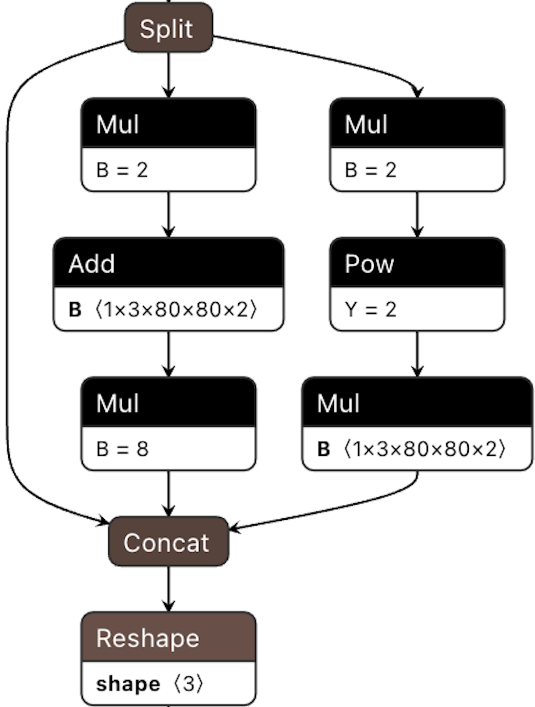
Therefore, the final verification result shows segmentation, as shown below:

  ====================================================================================
  Node                                    ON   Subgraph  Type
  -------------------------------------------------------------------------------------
  Reshape_199                             BPU  id(0)     Reshape
  Transpose_200                           BPU  id(0)     Transpose
  Sigmoid_201                             BPU  id(0)     HzLut
  Split_202                               BPU  id(0)     Split
  Mul_204                                 CPU  --        Mul
  Add_206                                 CPU  --        Add
  Mul_208                                 CPU  --        Mul
  Mul_210                                 CPU  --        Mul
  Pow_211                                 BPU  id(1)     HzLut
  Mul_213                                 CPU  --        Mul
  Concat_214                              CPU  --        Concat
  Reshape_215                             CPU  --        Reshape
  Conv_216                                BPU  id(0)     HzSQuantizedConv
  Reshape_217                             BPU  id(0)     Reshape
  Transpose_218                           BPU  id(0)     Transpose
  Sigmoid_219                             BPU  id(0)     HzLut
  Split_220                               BPU  id(0)     Split
  Mul_222                                 CPU  --        Mul
  Add_224                                 CPU  --        Add
  Mul_226                                 CPU  --        Mul
  Mul_228                                 CPU  --        Mul
  Pow_229                                 BPU  id(2)     HzLut
  Mul_231                                 CPU  --        Mul
  Concat_232                              CPU  --        Concat
  Reshape_233                             CPU  --        Reshape
  Conv_234                                BPU  id(0)     HzSQuantizedConv
  Reshape_235                             BPU  id(0)     Reshape
  Transpose_236                           BPU  id(0)     Transpose
  Sigmoid_237                             BPU  id(0)     HzLut
  Split_238                               BPU  id(0)     Split
  Mul_240                                 CPU  --        Mul
  Add_242                                 CPU  --        Add
  Mul_244                                 CPU  --        Mul
  Mul_246                                 CPU  --        Mul
  Pow_247                                 BPU  id(3)     HzLut
  Mul_249                                 CPU  --        Mul
  Concat_250                              CPU  --        Concat
  Reshape_251                             CPU  --        Reshape
  Concat_252                              CPU  --        Concat

Note: This log output is for illustration only. In practice, please refer to the actual log output from your tool version.

According to the hints provided by hb_mapper checker, operators running on the BPU generally achieve better performance. CPU operators such as pow and reshape can be removed from the model, and their functionality moved to post-processing, thereby reducing the number of subgraphs.

While multiple subgraphs do not block the conversion process, they significantly impact model performance. It is recommended to adjust model operators to execute on the BPU whenever possible. You can refer to the BPU operator support list in the X5 processor operator support list for functionally equivalent operator replacements, or move CPU operators in the model to pre- or post-processing stages for CPU computation.

6.3.2.4. Model Conversion

The model conversion stage transforms the floating-point model into an X5 mixed heterogeneous model. After this stage, you will obtain a model that can run on the X5 processor. Before conversion, ensure you have successfully passed the previous model verification step.

Model conversion is performed using the hb_mapper makertbin tool, which completes critical processes such as model optimization and calibration quantization. Calibration requires preparation of calibration data according to the model’s preprocessing requirements. To help you fully understand model conversion, this section will sequentially cover calibration data preparation, tool usage, internal conversion process explanation, result interpretation, and output artifact interpretation.

Preparing Calibration Data

During model conversion, the calibration phase requires approximately 100 calibration samples, each as a separate data file. To ensure accuracy after conversion, we recommend that these calibration samples come from your model’s training or validation set, avoiding rare or abnormal samples such as solid-color images or images without any detection or classification targets.

The preprocess_on parameter in the conversion configuration file corresponds to two different preprocessing sample requirements depending on whether it is enabled or disabled. (For detailed parameter configuration, refer to the relevant explanation in the calibration parameter group below.) When preprocess_on is disabled, you must apply the same preprocessing to samples from the training/validation set as done before model inference (inference). The processed calibration samples will have the same data type (input_type_train), dimensions (input_shape), and layout (input_layout_train) as the original model. For models with featuremap inputs, you can use the numpy.tofile command to save the data as a float32 binary file. The toolchain will read the data during calibration using the numpy.fromfile command. For example, an original floating-point classification model trained on ImageNet has only one input node, with input specifications as follows:

Input type: BGR
Input layout: NCHW
Input dimensions: 1x3x224x224

Data preprocessing when using the validation set for model inference (inference) includes:

Scale image proportionally so the shorter side is 256.
Use the center_crop method to extract a 224x224 image.
Subtract mean per channel.
Multiply data by a scale factor.

Sample processing code for the above example model:

To avoid excessive code length, simple transformer implementation code is not included. For specific usage, please refer to the Transformer Usage Guide section.

Tip:

It is recommended to refer to preprocessing methods in the horizon_model_convert_sample example package of the X5 algorithm toolchain, such as 02_preprocess.sh and preprocess.py for Caffe and ONNX example models.

# This example uses skimage; OpenCV usage may differ
# Note: The transformers below do not include mean subtraction or scaling
# Mean and scale operations are fused into the model; refer to norm_type/mean_value/scale_value configuration below
def data_transformer():
    transformers = [
    # Scale proportionally, short side to 256
    ShortSideResizeTransformer(short_size=256),
    # CenterCrop to get 224x224 image
    CenterCropTransformer(crop_size=224),
    # skimage reads as NHWC, convert to NCHW required by model
    HWC2CHWTransformer(),
    # skimage reads RGB, convert to BGR required by model
    RGB2BGRTransformer(),
    # skimage values in [0.0,1.0], adjust to model's required range
    ScaleTransformer(scale_value=255)
    ]

    return transformers

# src_image: original image from calibration set
# dst_file: filename for storing final calibration data
def convert_image(src_image, dst_file, transformers):
    image = skimage.img_as_float(skimage.io.imread(src_image))
    for trans in transformers:
        image = trans(image)
    # Model specifies input_type_train BGR as UINT8
    image = image.astype(np.uint8)
    # Save calibration sample as binary data file
    image.tofile(dst_file)

if __name__ == '__main__':
    # Pseudocode: collection of original calibration images
    src_images = ['ILSVRC2012_val_00000001.JPEG', ...]
    # Pseudocode: final calibration filenames (extension not restricted)
    # calibration_data_bgr_f32 is the cal_data_dir specified in your config file
    dst_files = ['./calibration_data_bgr_f32/ILSVRC2012_val_00000001.bgr', ...]

    transformers = data_transformer()
    for src_image, dst_file in zip(src_images, dst_files):
        convert_image(src_image, dst_file, transformers)

Tip:

When preprocess_on is enabled, calibration samples can be image files in formats supported by skimage.
The conversion tool reads these images and resizes them to the size required by the model’s input node, using the result as calibration input.
This approach is simpler but does not guarantee quantization accuracy. Therefore, we strongly recommend using the disabled preprocess_on method.

Note:

The input_shape parameter in the YAML file specifies the input data dimensions of the original floating-point model. For dynamic input models, this parameter sets the converted input size. Calibration data shape must match input_shape.
For example, if the original floating-point model’s input node shape is ?x3x224x224 (”?” is a placeholder indicating the first dimension is dynamic), and input_shape: 8x3x224x224 is set in the conversion configuration file, each calibration data sample should be 8x3x224x224. (Please note: Models with input shape first dimension not equal to 1 do not support modifying batch information via the input_batch parameter.)

Using the hb_mapper makertbin Tool for Model Conversion

The hb_mapper makertbin tool provides two modes: with or without the fast-perf mode.

When fast-perf mode is enabled, the tool generates a bin model capable of achieving maximum performance on the target device. Internally, the tool performs the following operations:

Executes BPU-compatible operators on the BPU whenever possible (for X5, operators to run on BPU can be specified via the node_info parameter in the YAML file).
Removes non-essential CPU operators at the model’s beginning and end, including: Quantize/Dequantize, Transpose, Cast, Reshape, etc.
Compiles the model using the highest-performance O3 optimization level.

Tip:

It is recommended to refer to script methods in the horizon_model_convert_sample example package of the X5 algorithm toolchain, such as 03_build.sh for Caffe and ONNX example models.

Usage of the hb_mapper makertbin command:

Without fast-perf mode:

hb_mapper makertbin --config ${config_file}  \
                    --model-type  ${model_type}

With fast-perf mode:

hb_mapper makertbin --fast-perf --model ${caffe_model/onnx_model} --model-type ${model_type} \
                    --proto ${caffe_proto} \
                    --march ${march}

Note: If you enable fast-perf mode, since the tool uses built-in high-performance configurations, do not configure the --config parameter.

Explanation of hb_mapper makertbin parameters:

--help
Display help information and exit.

-c, --config
Configuration file for model compilation, in YAML format with a .yaml extension. Refer to the complete template in the following section.

--model-type
Specifies the type of input model for conversion. Currently supports caffe or onnx.

--fast-perf
Enables fast-perf mode. When enabled, the tool generates a bin model capable of maximum performance on the target device, suitable for subsequent performance evaluation.

If fast-perf mode is enabled, the following configurations are also required:

--model
Caffe or ONNX floating-point model file.

--proto
Specifies the Caffe model’s prototxt file.

--march
BPU microarchitecture. For X5, set to bayes-e.

-i, --input-shape Optional parameter to specify the input node’s shape information. Currently only effective when fast-perf is enabled. Usage:

Specify shape for a single input node: --input-shape input_1 1x3x224x224.
Specify shapes for multiple input nodes: --input-shape input_1 1x3x224x224 --input-shape input_2 1x3x224x224.

Note: If the --input-shape parameter is not specified, the tool only supports models with dynamic input nodes whose first dimension is [-1, 0, ?], defaulting to setting the first dimension to 1.

The generated log file is stored in the command execution path, named hb_mapper_makertbin.log.

Note:

For X5 YAML configuration files, you can directly use the Caffe Model Quantization YAML File Template and X5 ONNX Model Quantization YAML Template.
If the hb_mapper makertbin step terminates abnormally or produces error messages, the model conversion has failed. Check the terminal output or the hb_mapper_makertbin.log log file in the current directory for error details and suggested fixes. If the issue persists, contact technical support or post your question on the Official Technical Community. We will provide support within 24 hours.

Model Conversion YAML Configuration Parameters

Note:

Either a Caffe model or an ONNX model must be specified. Choose either caffe_model + prototxt or onnx_model, but not both.

# Model Parameters Group
model_parameters:
  # Original Caffe floating-point model description file
  prototxt: '***.prototxt'

  # Original Caffe floating-point model data file
  caffe_model: '****.caffemodel'

  # Original ONNX floating-point model file
  onnx_model: '****.onnx'

  # Target processor architecture for conversion, keep default
  march: 'bayes-e'

  # Prefix name for the output model file used on the target device
  output_model_file_prefix: 'mobilenetv1'

  # Directory for storing conversion output results
  working_dir: './model_output_dir'

  # Specify whether the converted mixed heterogeneous model retains the ability to output intermediate results of each layer; keep default
  layer_out_dump: False

  # Specify the model's output nodes
  output_nodes: {OP_name}

  # Batch remove nodes of a specific type
  remove_node_type: Dequantize

  # Remove nodes with specified names
  remove_node_name: {OP_name}

# Input Information Parameters Group
input_parameters:
  # Input node name of the original floating-point model
  input_name: "data"

  # Input data format of the original floating-point model (number/order matches input_name)
  input_type_train: 'bgr'

  # Input data layout of the original floating-point model (number/order matches input_name)
  input_layout_train: 'NCHW'

  # Input data dimensions of the original floating-point model
  input_shape: '1x3x224x224'

  # Batch size actually input to the network during execution, default is 1
  input_batch: 1

  # Preprocessing method added to input data in the model
  norm_type: 'data_mean_and_scale'

  # Mean values subtracted from images in preprocessing method; use spaces to separate values for per-channel means
  mean_value: '103.94 116.78 123.68'

  # Scaling factor for images in preprocessing method; use spaces to separate values for per-channel scaling
  scale_value: '0.017'

  # Input data format adapted by the converted mixed heterogeneous model (number/order matches input_name)
  input_type_rt: 'yuv444'

  # Special format for input data
  input_space_and_range: 'regular'

  # Input data layout adapted by the converted mixed heterogeneous model (number/order matches input_name); not required if input_type_rt is set to nv12
  input_layout_rt: 'NHWC'
 # Calibrate parameter group
  calibration_parameters:
  # The storage directory of calibration samples used for model calibration
  cal_data_dir: './calibration_data'

  # Specify the data storage type of the calibration data binary file.
  cal_data_type: 'float32'

  # Turn on automatic processing of picture calibration samples (skimage read; resize to input node size)
  #preprocess_on: False
  
  # The type of algorithm used to calibrate, the default calibration algorithm used first
  calibration_type: 'default'

  # max calibration method parameters
  # max_percentile: 1.0

  # Force specify that the OP runs on the CPU, generally does not require configuration. This function can be enabled during the model accuracy tuning stage to try precision optimization.
  #run_on_cpu: {OP_name}

  # Force specify that the OP runs on the BPU, generally does not require configuration. This function can be enabled during the model performance tuning stage to try performance optimization.
  # run_on_bpu: {OP_name}
# Specify whether to calibrate for each channel
  #per_channel: False

  # Specify the data accuracy of the output node
  #optimization: set_model_output_int8

# Compile parameter group
compiler_parameters:
  # Compile policy selection
  compile_mode: 'lateency'

  # Whether to turn on the compiled debug information, keep the default False
  debug: False

  # Number of cores running on the model
  core_num: 1

  # Select the optimization level of model compilation, keep the default O3
  optimize_level: 'O3'

  # Specify the source of input data with the name data
  #input_source: {"data": "pyramid"}

  # Specify the maximum continuous execution time for each function call of the model
  #max_time_per_fc: 1000

  # Specify the number of processes when compiling the model
  #jobs: 8

# This parameter group does not require configuration and is only enabled when there is a custom CPU operator.
#custom_op:
# Customize the calibration method of the op, it is recommended to use the registration method register
  #custom_op_method: register

  # Custom OP implementation file, multiple files can be separated by ";" and the file can be generated by templates. For details, please refer to the related documents of Custom OP
  #op_register_files: sample_custom.py

  # Customize the folder where the OP implements the file is located, please use the relative path
  #custom_op_dir: ./custom_op

The configuration file mainly includes model parameter group, input information parameter group, calibration parameter group and compile parameter group. In your configuration file, all four parameter group positions need to exist. The specific parameters are divided into optional and required. The optional parameters can be not configured.

The specific parameter setting form is: param_name: 'param_value' ; If there are multiple values in the parameter, each value is separated by using the ';' symbol: param_name: 'param_value1; param_value2; param_value3' ; for the specific configuration method, please refer to: run_on_cpu: 'conv_0; conv_1; conv12' .

Tips:

When the model is a multi-input model, it is recommended that the user explicitly write out optional parameters (input_name, input_shape, etc.) to avoid errors in the corresponding order of parameters.
When configuring march to bayes-e, that is, when performing X5 model conversion, if you configure optimization_level to O3, hb_mapper makertbin provides caching capability by default. That is, when you use hb_mapper makertbin to compile the model for the first time, a cache file will be automatically created. In the future, when your working_dir remains unchanged, this file will be automatically called during repeated compilation, reducing your compilation time.

Notice:

Note that if input_type_rt is set to nv12 or yuv444, then odd number cannot appear in the input size of the model.
After the model conversion is successful, if an OP that meets the X5BPU operator constraints still runs on the CPU, the main reason is that the OP belongs to the passive quantization OP. For content related to passive quantization, please read the Active Quantization and Passive Quantization Logic in the Algorithm Tool Chain chapter.

The following is the specific parameter information, there will be more parameters, we will introduce it according to the above parameter group order.

Model parameter group

Parameter name	Parameter configuration description	Value range description	Optional/required
`prototxt`	Parameter function: Specify the prototxt file name of the Caffe floating point model. Particle Description: Must be configured when the `model-type` of `hb_mapper maketbin` is `caffe`.	Value range: None. Default configuration: None.	Optional
`caffe_model`	Parameter function: Specify the name of the caffemodel file of the Caffe floating point model. Particle Description: Must be configured when the `model-type` of `hb_mapper maketbin` is `caffe`.	Value range: None. Default configuration: None.	Optional
`onnx_model`	Parameter function: Specify the name of the onnx file of the ONNX floating point model. Particle Description: It must be configured when the `model-type` of `hb_mapper maketbin` is `onnx`.	Value range: None. Default configuration: None.	Optional
`march`	Parameter function: Specify the platform architecture that needs to be supported for outputting hybrid heterogeneous models. Particle description: Configure the BPU microframework of X5.	Value range: `bayes-e`. Default configuration: None.	Required
`output_model_file_prefix`	Parameter function: Specifies the name prefix for the conversion to produce a hybrid heterogeneous model. Parameter description: The name prefix of the output fixed-point model file.	Value range: None. Default configuration: None.	Required
`working_dir`	Parameter function: Specifies the directory where the result of the model conversion output is stored. Parameter description: If the directory does not exist, the tool will automatically create the directory.	Value range: None. Default configuration: `model_output`.	Optional
`layer_out_dump`	Parameter function: Specifies whether the hybrid heterogeneous model retains the ability to output intermediate layer values. Parameter description: The output value of the intermediate layer is a means required for debugging. Please do not turn it on in normal state.	Value range: `True`, `False`. Default configuration: `False`.	Optional
`output_nodes`	Parameter function: Specify the output node of the model. Parameter description: Generally, the conversion tool will automatically identify the output node of the model. This parameter is used to support you specifying some intermediate levels as output. To set the value to the specific node name in the model, please refer to the configuration description of the `param_value` configuration for multiple values. It should be noted that once this parameter is set, the tool will no longer automatically recognize the output nodes, and the nodes you specify through this parameter are all outputs.	Value range: None. Default configuration: None.	Optional
`remove_node_type`	Parameter function: Set the type of delete node. Particle Description: This parameter is a hidden parameter. If it is not set or set to empty, it will not affect the model conversion process. This parameter is used to support you to set the type information of the node to be deleted. The deleted node must be connected to the input or output of the model at the beginning or end of the model. Note: The nodes to be deleted will be deleted in sequence and the model structure will be dynamically updated; at the same time, before the node is deleted, it will also be judged whether the node is located at the input and output of the model. Therefore, the order of deleting nodes is very important.	Value range: "Quantize", "Transpose", "Dequantize", "Cast", "Reshape". Different types are divided by ";". Default configuration: None.	Optional
`remove_node_name`	Parameter function: Set the name of the delete node. Particle Description: This parameter is a hidden parameter. Not setting or setting to empty will not affect the model conversion process. This parameter is used to support you to set the name of the node to be deleted. The deleted node must be connected to the input or output of the model at the beginning or end of the model. Note: The nodes to be deleted will be deleted in sequence and the model structure will be dynamically updated; at the same time, before the node is deleted, it will also be judged whether the node is located at the input and output of the model. Therefore, the order of deleting nodes is very important.	Value range: None. Different types are divided by ";". Default configuration: None.	Optional
`set_node_data_type`	Parameter function: Configure the output data type of the specified op to be int16, this parameter only supports X5 configuration! Parameter description: During the model conversion process, the default input and output data type of most ops is int8. This parameter can be used to specify that the output data type of a specific op is int16 (under certain constraints). Int16 details are described in the X5 int16 Configuration Notes section. Note: This parameter-related function has been merged into the `node_info` parameter.	Value range: Support the operator range of int16. You can refer to the X5 operator support constraint list in Model operator support list. Default configuration: None.	Optional
`debug_mode`	Parameter function: Save calibration data for precision debug analysis. Parameter description: This parameter is used to save calibration data for precision debug analysis, and the data format is .npy. This data can be sent directly to the model for inference through np.load(). If you do not set this parameter, you can also save the data yourself and use the precision debug tool for accuracy analysis.	Value range: ``"dump_calibration_data"``` Default configuration: None.	Optional
`node_info`	Parameter function: Supports configuration of the input and output data type of the specified OP to be int16 and forcing the specified operator to run on the CPU or BPU. This parameter only supports X5 configuration! Parameter description: Based on the principle of reducing parameters in yaml, we incorporate the capabilities of the three parameters `set_node_data_type`, `run_on_cpu` and `run_on_bpu` into this parameter, and on this basis, we expand the ability to configure the specified op input data type to int16. `node_info` Parameter usage method: -Only specify that the OP runs on the BPU/CPU (see BPU as an example, the CPU method is the same): node_info: { "node_name": { 'ON': 'BPU', } } -Configure only node data types: node_info: 'node_name1:int16;node_name2:int16' For multiple values, please refer to `param_value configuration <param_value>`. -Specify that the OP runs on the BPU and configures the input and output data type of the OP: node_info: { "node_name": { 'ON': 'BPU', 'InputType': 'int16', 'OutputType': 'int16' } } 'InputType': 'int16' means that all input data types of the specified operator are int16. If you need to specify the InputType for the operator specific input, you can configure it by specifying the number after the InputType. For example: 'InputType0': 'int16' means that the first input data type of the specified operator is int16, 'InputType1': 'int16' means that the second input data type of the specified operator is int16, and so on. Note: 'OutputType' does not support OutputType that specifies the specific output of the operator. It takes effect on all outputs of the operator after configuration. It does not support the configuration of 'OutputType0', 'OutputType1', etc.	Value range: Support the operator range of int16. You can refer to the X5 operator support constraint list in Model Operator Support List. You can specify that the operators running on the CPU or BPU must be the operators included in the model. Default configuration: None.	Optional

Enter information parameter group

Parameter name	Parameter configuration description	Value range description	Optional/required
`input_name`	Parameter function: Specifies the input node name of the original floating point model. Parameter description: There is no need to configure when the floating point model has only one input node. More than one input node must be configured to ensure the accuracy of subsequent types and calibration data input order. For configuration methods for multiple values, please refer to the previous description of param_value configuration.	Value range: None. Default configuration: None.	Optional
`input_type_train`	Parameter function: Specifies the input data type of the original floating point model. Parameter description: Each input node needs to configure a certain input data type. When multiple input nodes exist, the set node order needs to be strictly consistent with the order in `input_name`. For configuration methods for multiple values, please refer to the previous article for the configuration description of the `param_value` configuration. For the selection of data types, please refer to the introduction of the following section: Interpretation of the internal process of conversion.	Value range: `rgb`, `bgr`, `yuv444`, `gray`, `featuremap`. Default configuration: None.	Required
`input_layout_train`	Parameter function: Specifies the input data layout of the original floating point model. Parameter description: Each input node needs to configure a certain input data arrangement, which must be the same as the data arrangement used in the original floating-point model. When multiple input nodes exist, the set node order needs to be strictly consistent with the order in `input_name`. For configuration methods for multiple values, please refer to the previous article for the configuration description of the `param_value` configuration. For what is data layout, please refer to: Interpretation of the internal process of conversion.	Value range: NHWC, NCHW. Default configuration: None.	Required
`input_type_rt`	Parameter function: The input data format that needs to be adapted for hybrid heterogeneous models after conversion. Parameter description: Here is the data format you need to use. It does not require that it is consistent with the data format of the original model, but it should be noted that the data fed to the model on the platform is used in this format. Each input node needs to configure a certain input data type. When multiple input nodes exist, the set node order needs to be strictly consistent with the order in `input_name`. For configuration methods for multiple values, please refer to the previous article for the configuration description of the `param_value` configuration. For the selection of data types, please refer to the introduction of the following section: Interpretation of the internal process of conversion.	Value range: `rgb`, `bgr`, `yuv444`, `nv12`, `gray`, `featuremap`. Default configuration: None.	Required
`input_layout_rt`	Parameter function: The input data layout that needs to be adapted for the hybrid heterogeneous model after conversion. Parameter description: Each input node needs to configure a certain input data arrangement, which is the arrangement you want to specify for the hybrid heterogeneous model. Inappropriate input data arrangement settings will affect performance. If input_type_rt is configured as nv12, the parameters here do not need to be configured. When multiple input nodes exist, the set node order needs to be strictly consistent with the order in `input_name`. For configuration methods for multiple values, please refer to the previous article for the configuration description of the `param_value` configuration. For what is data layout, please refer to: Interpretation of the internal process of conversion.	Value range: `NCHW`, `NHWC`. Default configuration: None.	Optional
`input_space_and_range`	Parameter function: Specify a special format for input data format. Particle Description: This parameter is to adapt to the yuv420 format output by different ISPs. This configuration is only valid when the corresponding input_type_rt is nv12. regular is the common yuv420 format, with a numerical range of [0,255]; bt601_video is another video format, yuv420, with a numerical range of [16,235]. For more information, you can learn about bt601 through the network information. You do not configure this parameter without explicitly needed.	Value range: `regular`, `bt601_video`. Default configuration: `regular`.	Optional
`input_shape`	Parameter function: Specifies the input data size of the original floating point model. Parameter description: Several dimensions of shape are connected in x, such as 1x3x224x224. The original floating-point model can not be configured when there is only one input node, and the tool will automatically read the dimension information in the model file. When configuring multiple input nodes, the set node order needs to be strictly consistent with the order in `input_name`. For configuration methods for multiple values, please refer to the previous article for the configuration description of the `param_value` configuration.	Value range: None. Default configuration: None.	Optional
`input_batch`	Parameter function: Specifies the number of input batches that need to be adapted to the hybrid heterogeneous model after conversion. Parameter description: Here input_batch is the number of input batches input to the hybrid heterogeneous bin model after conversion, but it does not affect the number of input batches input to the onnx model after conversion. This parameter only supports configuring one numerical value. When the model is multi-input, this value will act on all inputs of the model. This parameter defaults to 1 if it is not configured. This parameter can only be used when the first dimension of `input_shape` is 1. When the model is multi-input, the first dimension of `input_shape` that requires all inputs is 1. This parameter will only take effect if the original onnx model itself supports multi-batch inference. This parameter can only be effective if the original onnx model itself supports multi-batch inference. However, due to the complexity of the operator, if during the model conversion process, if you encounter a prompt that the model does not support configuring the input_batch parameter, please try to directly export a multi-batch onnx model and correctly configure the calibration data size to re-convert (this parameter is no longer necessary to configure this parameter).	Value range: `1-4096`. Default configuration: `1`.	Optional
`norm_type`	Parameter function: Preprocessing method for input data added to the model. Parameter description: `no_preprocess` means no data preprocessing is added; `data_mean` means providing a mean reduction preprocessing; `data_scale` means providing a scale coefficient preprocessing; `data_mean_and_scale` means providing a scale coefficient preprocessing first and then multiplying the scale coefficient preprocessing. When there are more than one node when entering the input, the set node order needs to be strictly consistent with the order in `input_name`. For configuration methods for multiple values, please refer to the previous article for the configuration description of the `param_value` configuration. For the impact of configuring this parameter, please refer to the introduction of the: Interpretation of the internal process of conversion.	Value range: `data_mean_and_scale`, `data_mean`, `data_scale`, `no_preprocess`. Default configuration: None.	Required
`mean_value`	Parameter function: Specifies the mean value of the image subtraction of the preprocessing method. Particle Description: This parameter needs to be configured when `norm_type` exists `data_mean_and_scale` or data_mean. For each input node, there are two configuration methods. The first is to configure only one value to subtract this mean for all channels; the second is to provide values consistent with the number of channels (these values are separated by spaces), indicating that each channel will subtract a different mean. The number of input nodes configured must be consistent with the number of nodes configured by norm_type. If there is a node that does not require mean processing, configure `'None'` for that node. For configuration methods for multiple values, please refer to the previous article for the configuration description of the `param_value` configuration.	Value range: None. Default configuration: None.	Optional
`scale_value`	Parameter function: Specify the numerical scale coefficient of the preprocessing method. Particle Description: This parameter needs to be configured when `norm_type` exists `data_mean_and_scale` or `data_scale`. For each input node, there are two configuration methods. The first is to configure only one value, which means that all channels are multiplied by this coefficient; the second is to provide values consistent with the number of channels (these values are separated by spaces), which means that each channel is multiplied by a different coefficient. The number of input nodes configured must be consistent with the number of nodes configured in `norm_type`. If there is a node that does not require scale`processing, then configure`'None'`for that node. For configuration methods for multiple values, please refer to the previous article for the configuration description of`param_value``.	Value range: None. Default configuration: None.	Optional

input_type_rt/input_type_train additional instructions:

X5’s computing platform architecture has made two assumptions in order to improve performance during design:

Assume that the input data is all quantized int8.
The data obtained by the camera is nv12.

Therefore, if you use the rgb (NCHW) input format when training the model, but want to make this model efficiently process nv12 data, you only need to do the following configuration when converting the model:

  input_parameters:
      input_type_rt: 'nv12'
      input_type_train: 'rgb'
      input_layout_train: 'NCHW'

Tips:

If you use the gray format when training the model, and the data input in actual use is nv12 format, you can configure both input_type_rt and input_type_train during model conversion to gray. When developing embedded applications, only use the y-channel address of nv12 as input.

Calibration parameter group

Parameter name	Parameter configuration description	Value range description	Optional/required
`cal_data_dir`	Parameter function: Specifies the directory of the calibration samples used for model calibration. Particle Description: The calibration data in the directory must meet the requirements of the input configuration. For details, please refer to the introduction in the Preparation of Calibration Data section. When configuring multiple input nodes, the set node order needs to be strictly consistent with the order in `input_name`. For configuration methods for multiple values, please refer to the previous article for the configuration description of `param_value`. When the calibration_type is `load`, `skip`, cal_data_dir does not need to be filled in. Note: For your convenience, if the configuration of cal_data_type is not found, we will configure the data type according to the folder suffix. If the folder suffix ends with `_f32`, the data type is considered float32, otherwise the data type is considered uint8. Of course, we strongly recommend that you constrain your data types via the cal_data_type parameter.	Value range: None. Default configuration: None.	Calibration_type is required when loading or skip
`cal_data_type`	Parameter function: Specifies the data storage type of the calibration data binary file. Parameter description: Specifies the data storage type of the binary file used during model calibration. If there is no specified value, the folder name suffix will be used to make judgments.	Value range: `float32`, `uint8`, `int32`, `int16`, `int8`. Default configuration: None.	Optional
`preprocess_on`	Parameter function: Turn on automatic processing of picture calibration samples. Parameter description: This option is only applicable to models with 4-dimensional image input. Do not turn on this option for non-4-dimensional models. When starting this function, the cal_data_dir directory stores image data such as jpg/bmp/png. The tool will use skimage to read the image and resize to the size required by the input node. To ensure the calibration effect, it is recommended that you keep this parameter off. Please refer to the introduction in the Preparation of Calibration Data section for the impact of use.	Value range: `True`, `False`. Default configuration: `False`.	Optional
`calibration_type`	Parameter function: The type of algorithm used to calibrate. Parameter description: Each `kl` and `max` are public calibration quantization algorithms, and their basic principles can be viewed through network data. When calibrating using the `load` method, the qat model must be a model derived through plugin. `mix` is a search strategy that integrates multiple calibration methods. It can automatically determine quantified sensitive nodes and select the best methods from different calibration methods on the node granularity, and ultimately build a combined calibration method that integrates the advantages of multiple calibration methods. `default` is an automatic search strategy that will try to obtain a relatively good combination from the series calibration quantization parameters. It is recommended that you try `default` first. If the final accuracy result does not meet expectations, it is recommended to configure different calibration parameters according to the Accuracy Tuning section. If you just want to try to verify the performance of the model but have no requirements for accuracy, you can try the "skip" method for calibration. This method uses random numbers for calibration, and you do not need to prepare calibration data, which is more suitable for first attempts to verify the model structure. Note: When using skip method, the obtained model cannot be used for accuracy verification because of the random number calibration.	Value range: `default`, `mix`, `kl`, `max`, `load` and `skip`. Default configuration: `default`.	Required
`max_percentile`	Parameter function: This parameter is the parameter of the `max` calibration method, which is used to adjust the intercept point of the `max` calibration. Particle Description: This parameter is only valid when `calibration_type` is `max`. Common configuration options are: 0.99999/0.99995/0.99990/0.99950/0.99900. It is recommended that you try the `calibration_type` configuration `default` first. If the final accuracy result does not meet expectations, it is recommended to adjust the parameter according to the accuracy tuning section.	Value range: `0.5`~`1.0`. Default configuration: `1.0`.	Optional
`per_channel`	Parameter function: Controls whether to calibrate each channel of featuremap. Parameter description: `calibration_type` is valid when setting non-default. It is recommended that you try `default` first. If the final accuracy result does not meet expectations, it is recommended to adjust the parameter according to the accuracy tuning section.	Value range: `True`, `False`. Default configuration: `False`.	Optional
`run_on_cpu`	Parameter function: Force the specified operator to run on the CPU. Parameter description: Although the performance on the CPU is not as good as the BPU, it provides float accuracy calculation. If you are sure that some operators need to be calculated on the CPU, you can specify this parameter. To set the value to the specific node name in the model, please refer to the configuration description of the `param_value` configuration for multiple values. Note: The relevant functions of this parameter in X5**have been merged into the `node_info` parameter.	Value range: None. Default configuration: None.	Optional
`run_on_bpu`	Parameter function: Force the OP to run on the BPU. Parameter description: In order to ensure the accuracy of the final quantization model, in some cases, the conversion tool will run some operators with BPU calculation conditions on the CPU. If you have high performance requirements and are willing to pay more quantization losses, you can use this parameter to clearly specify the operator to run on the BPU. The setting value is the specific node name in the model. For the configuration method of multiple values, please refer to the previous article for the configuration description of the `param_value` configuration. Note: The relevant functions of this parameter in X5**have been merged into the `node_info` parameter.	Value range: None. Default configuration: None.	Optional
`optimization`	Parameter function: Make the model output in int8/int16 format. Parameter description: -When the value is specified as set_model_output_int8, set the model to the low-precision output in the int8 format; -When the value is specified as set_model_output_int16, set the model to the low-precision output in the int16 format; -When the value is specified as set_{NodeKind}_input_int16, a certain type of operator input in the model will be quantized into int16. If the node context does not support int16, the int8 calculation will be backed up and the log will be printed; -When the specified value is set_{NodeKind}_output_int16, the output of a certain type of operator in the model will be quantized into int16. If the node context does not support int16, the calculation of int8 will be backed up and the log will be printed; -When the specified value is set_Softmax_input_int8/set_Softmax_output_int8, since the current softmax defaults to float to calculate non-quantized nodes, these two specified values will quantize the softmax operator into int8 and calculate on the BPU. There is no difference between the two in use; -When the specified value is asymmetric, asymmetric quantization will be attempted to enable asymmetric quantization, which can improve the quantization accuracy on some models. When the calibration_type is configured as default, This parameter will be automatically selected by the algorithm, and it cannot be configured explicitly at this time; -When the value is specified as bias_correction, the BiasCorrection quantization method can be used to improve the quantization accuracy on some models; -When the value is specified as lstm_batch_last, for X5 BPU, when the batch-input size of LSTM is large, the batch dimension can be converted to W dimension for calculation (guarantee equivalence), which is more in line with the hardware calculation logic. In some scenarios, the effect of acceleration of X5 BPU inference performance can be achieved; Since the inference performance of the model deployment is related to optimization of multiple levels, *Therefore, this method cannot guarantee that performance acceleration can be achieved.	Value range: `set_model_output_int8`, `set_model_output_int16`, `set_{NodeKind}_input_int16`, `set_{NodeKind}_output_int16`, `set_Softmax_input_int8`, `asymmetric`, `bias_correction`, `lstm_batch_last` Note: Here NodekindFor standard ONNX operator types, such as Conv, Mul, Sigmoid, etc. (case sensitive), please refer to the onnx official op document or Model operator support list. Default configuration: None.	Optional

preprocess_on supplementary notes:

If you specify the configuration parameter preprocess_on=True:

The tool can automatically complete the preprocessing of calibration pictures through the setting preprocess_on to True. In this mode, you need to specify the storage path for the calibration JPEG picture in cal_data_dir. When the model is calibrated, the JPEG picture read in the skimage method inside the tool will scale the picture to the input_shape specified in the configuration file through skimage resize. And adjust the image format to the format specified by input_type_rt.

For example, if the input JPEG image size is 608x608, the image is scaled to 224x224 after the default preprocessing. The memory format of the image is adjusted to the bgr(NCHW) format, and the pixel value is adjusted to the range 0-255.

For default preprocessing, please refer to the following code:
```
def data_transformer(norm_type, input_dim, input_type_train):
image_width = input_dim[2]
          image_height = input_dim[1]
          transformers = [
              ResizeTransformer((image_height, image_width)),
              HWC2CHWTransformer(), # to CXHXW
              RGB2BGRTransformer(),
          ]

          transformers.append(ScaleTransformer(255))
```
If you specify configuration parameter preprocess_on=False:

You need to process the image yourself, process the image to the format specified in input_type_train, and save the data as a file in binary form. The format conversion from input_type_train to input_type_rt will be automatically added inside the tool.

Note: The file format is Row-major order.

Compile parameter group

Parameter name	Parameter configuration description	Value range description	Optional/required
`compile_mode`	Parameter function: Compile policy selection. Parameter description: `latency` aims to optimize inference time; `bandwidth` aims to optimize ddr's access bandwidth. If the model does not significantly exceed the expected bandwidth footprint, it is recommended that you use the `latency` strategy. `balance` Balances the optimization target latency and bandwidth. Set to this item to specify balance_factor.	Value range: `latency`, `bandwidth`, `'balance'`. Default configuration: `latency`.	Required
`balance_factor`	Parameter function: When compile_mode is specified as balance, it is used to specify the balance ratio. Particle Description: This parameter is only used when compile_mode is specified as balance, and the configuration does not take effect in other modes. -Configure 0 to be the best bandwidth, corresponding to the compilation strategy with compile_mode as bandwidth. -Configure 100 to achieve the best performance, corresponding to the compilation strategy with compile_mode latency.	Value range: `0-100`. Default configuration: None.	Required when compile_mode is balance
`debug`	Parameter function: Whether to open the compiled debug information. Parameter description: In the scenario where this parameter is enabled, the performance results of the static analysis of the model will be saved in the model. You can view the performance information of the model layer by layer BPU operator (including calculation amount, calculation time and data handling time) in the Layer Details tab. By default, it is recommended that you keep this parameter off.	Value range: `True`, `False`. Default configuration: `False`.	Optional
`core_num`	Parameter function: The number of cores running in the model. Parameter description: The X5 platform supports the use of multiple AI accelerator cores to complete a reasoning task at the same time. Multiple cores are suitable for situations with large input sizes. The dual-core speed in ideal state can reach about 1.5 times that of a single core. If your model input size is large and you have the ultimate pursuit of model speed, you can configure `core_num=2`. Note: X5This option only supports configuration as 1!	Value range: `1`, `2`. Default configuration: `1`.	Optional
`optimize_level`	Parameter function: Selection of optimization level for model compilation. Particle Description: The optional range of optimization level is `O0` ~ `O3`. `O0` does not do any optimization, the fastest compilation speed and the lowest optimization level. `O1` -`O3` As the optimization level increases, it is expected that the compiled model will be executed faster, but the compilation time will also become longer. For models that are normally used to generate and verify performance, `O3` level optimization must be used to ensure optimal performance. During certain process verification or precision debugging, you can try to speed up the process using lower-level optimization.	Value range: `O0`, `O1`, `O2`, `O3`. Default configuration: None.	Required
`input_source`	Parameter function: Set the input data source of the upper board bin model. Particle Description: This parameter is an option to adapt to the engineering environment. It is recommended that you have completed the model verification before configuring it. `ddr` means data comes from memory, `pyramid` and `resizer` mean fixed hardware on the processor. Note: If set to resizer, the h*w of the model must be less than 18432. How to adapt to the `pyramid` and `resizer` data sources in the engineering environment? This parameter configuration is a bit special. For example, if the model input name is data and the data source is memory (ddr), then the value should be configured here as `{"data": "ddr"}`.	Value range: `ddr`, `pyramid`, `resizer` Default configuration: None, default will be automatically selected from the optional range based on the value of input_type_rt.	Optional
`max_time_per_fc`	Parameter function: Specifies the maximum continuous execution time (units of us) for each function-call of the model. Parameter description: When the compiled data instruction model performs inference calculation on the BPU, it will be represented as a call of 1 or more function-calls (the execution granularity of the BPU). The value of 0 means no restrictions. This parameter is used to limit the maximum execution time of each function-call. The model has a chance to be preempted only when a single function-call is executed. For details, see the introduction in the Model Priority Control section. -This parameter is only used to implement the model preemption function, and can be ignored if this function is not required. -The model preemption function is only implemented on the development board side, and does not support the PC side emulator implementation.	Value range: `0 or 1000-4294967295`. Default configuration: `0`.	Optional
`jobs`	Parameter function: Set the number of processes when compiling the bin model. Parameter description: When compiling the bin model, it is used to set the number of processes. To a certain extent, it can improve the compilation speed.	Value range: `The maximum number of cores supported by the machine is within the range.` Default Configuration: None.	Optional
`advice`	Parameter function: Used to prompt the increase in time-consuming estimated after model compilation, in microseconds. Parameter description: During the compilation process of the model, time-consuming analysis will be performed inside the tool chain. In actual process, such as the operator performs data alignment operations, it will increase the time-consuming process. After setting this parameter, when the deviation between the actual calculation time and the theoretical calculation time-consuming of a certain OP is greater than the value you specified, the relevant log will be printed, including information about time-consuming changes, shape before and after data alignment, and padding ratio and other information.	Value range: Natural number. Default configuration: None. Not setting or setting to 0 means not turning on.	Optional

Custom operator parameter group

Parameter name	Parameter configuration description	Value range description	Optional/required
`custom_op_method`	Parameter function: Custom operator strategy selection. Parameter description: Currently only register policy is supported.	Value range: `register`. Default configuration: None.	Optional
`op_register_files`	Parameter function: Custom operator's Python implementation file name. Parameter description: Multiple files are available `;` separated	Value range: None. Default Configuration: None.	Optional
`custom_op_dir`	Parameter function: Custom operator's Python implementation file storage path. Particle Description: When setting the path, please use the relative path.	Value range: None. Default configuration: None.	Optional

X5 int16 configuration instructions

During the model conversion process, most operators in the model are quantized to int8 for calculation, and by configuring the node_info parameter, You can specify in detail that the input/output data type of an op is int16 calculation (for specific supported operator ranges, please refer to the X5 operator support list content in the Model Operator Support List. The basic principles are as follows:

After you configure an op input/output data type to int16, the model conversion will automatically update and check the op input/output context (context) int16 configuration. For example, when the input/output data type of op_1 is configured to be int16, the upper/next op of op_1 is actually potentially specified at the same time. For unsupported scenarios, the model conversion tool will print a log prompt that the int16 configuration combination is not supported for the time being and falls back to the int8 calculation.

Instructions for preprocessing HzPreprocess operator

The preprocessing HzPreprocess operator is a preprocessing operator node inserted after the model input node generated by the X5 algorithm toolchain model conversion tool during the model conversion process based on the yaml configuration file. It is used to normalize the input data of the model. This section mainly introduces the norm_type, mean_value, scale_value parameter variables and the generation of the model preprocessing HzPreprocess operator node.

norm_type parameter description:

Parameter function: This parameter is the preprocessing method of input data added in the model.
Parameter value range and description:
- no_preprocess means no data preprocessing is added.
- data_mean means to provide a mean-down preprocessing.
- data_scale means providing preprocessing of multiplication scale coefficients.
- data_mean_and_scale means to provide preprocessing of decreasing the mean first and then multiplying the scale coefficient.

Notice: When the input node is greater than one, the set node order needs to be strictly consistent with the order in input_name.

mean_value parameter description:

Parameter function: This parameter represents the mean of the image minus the specified preprocessing method.
Instructions for use: This parameter needs to be configured when the value of norm_type is data_mean_and_scale or data_mean.
Parameter description:
- When there is only one input node, only one value needs to be configured to indicate that all channels are subtracted from this mean.
- When there are multiple nodes, a value consistent with the number of channels is provided (these values are separated by spaces) indicating that each channel is subtracted from a different mean.

Notice:

The number of input nodes configured must be consistent with the number of nodes configured in norm_type.
If there is a node that does not require mean processing, configure 'None' for that node.

scale_value parameter description:

Parameter function: This parameter represents the numerical scale coefficient of the specified preprocessing method.
Instructions for use: This parameter needs to be configured when the value of norm_type is data_mean_and_scale or data_scale.
Parameter description:
- When there is only one input node, only one value needs to be configured to indicate that all channels are multiplied by this coefficient.
When there are multiple nodes, a value consistent with the number of channels is provided (these values are separated by spaces) indicating that each channel is multiplied by a different coefficient.

Notice:

The number of input nodes configured must be consistent with the number of nodes configured in norm_type.
If there is a node that does not require scale processing, configure 'None' for that node.

Calculation formulas and example description:

Calculation formula for data standardization processing during model training

The mean and scale parameters in the yaml file need to be converted to the mean and std during training.

The calculation method of standardized data operations in preprocessing nodes (i.e., the calculation formula in the HzPreprocess node) is norm\_data = ( data − means ) *scale.

Taking yolov3 as an example, the preprocessing code during training is:

def base_transform(image, size, mean, std):
    x = cv2.resize(image, (size, size).astype(np.float32))
    x /= 255
    x -= means
    x /= std
Return x

class BaseTransform:
    def __init__(self, size, mean=(0.406, 0.456, 0.485), std=(0.225, 0.224, 0.229)):
        self.size = size
        self.mean = np.array(mean, dtype=np.float32)
        self.std = np.array(std, dtype=np.float32)

Then the calculation formula is: $norm_data= (\frac{data}{255} −𝑚𝑒𝑎𝑛) *\frac{1}{𝑠𝑡𝑑}$,

The calculation method of rewritten to HzPreprocess node: $norm_data= (\frac{data}{255} −𝑚𝑒𝑎𝑛) *\frac{1}{𝑠𝑡𝑑} =(data−255𝑚𝑒𝑎𝑛) *\frac{1}{255𝑠𝑡𝑑}$ , Then: $mean_yaml = 255 means, 𝑠𝑐𝑎𝑙𝑒_𝑦𝑎𝑚𝑚𝑙= \frac{1}{255 𝑠𝑡𝑑}$ .

Calculation formulas during model inference

By using the configuration parameters in the yaml configuration file, decide whether to join the HzPreprocess node. When configuring mean/scale, when performing model conversion, a new HzPreprocess node will be added to the input end. The HzPreprocess node can be understood as a conv operation for the input data.

The calculation formula in HzPreprocess is: ((input(value range[-128,127]) + 128) -mean) *scale, where weight=scale, bias=(128-mean)*scale.

Notice:

After adding mean/scale in yaml, there is no need to add MeanTransformer and ScaleTransformer in preprocessing.
Add mean/scale to yaml and the parameters will be placed into the HzPreprocess node, which is a BPU node.

[Reference] Supported calibration methods

Currently we support the following calibration methods:

default default is an automatic search strategy that will try to obtain a relatively good combination from the series calibration quantization parameters.
mix mix is a search strategy that integrates multiple calibration methods, which can automatically determine quantized sensitive nodes and select the best method from different calibration methods on the node granularity. Finally, a combined calibration method is constructed that integrates the advantages of multiple calibration methods.
KL KL calibration method is borrowed from TensorRT’s solution, The KL entropy value is used to traverse the data distribution of each quantization layer, and the threshold is determined by finding the lowest KL entropy value. This method will lead to more data saturation and smaller data quantization granularity, and has better results than max calibration methods in some models with relatively concentrated data distribution.
max The max calibration method is to automatically select the maximum value in the quantization layer as the threshold during the calibration process. This method will lead to a larger granularity in data quantization, but it will also bring less number of saturation points than the KL method, and is suitable for neural network models with relatively discrete data distribution.
load

This parameter is required when using the model exported with QAT.
skip

If you just want to try to verify the performance of the model but have no requirements for accuracy, you can try the skip method for calibration. This method will use the random calibration data generated internally by max+ for calibration. You do not need to prepare calibration data, and it is more suitable for the first attempt to verify the model structure.

Note: It is important to note that when using the skip method, since this method uses the random calibration data generated internally by max+ for calibration, the resulting model cannot be used for accuracy verification.

Interpretation internal process

The model conversion stage completes the conversion of floating-point model to X5 hybrid heterogeneous model. In order to enable this heterogeneous model to run quickly and efficiently on the embedded end, the focus of model conversion is to solve the two problems of input data processingand model optimization and compilation. This section will focus on these two key problems in turn. Input Data ProcessingThe X5 processor will provide hardware-level support solutions for certain specific types of model input paths. For example: the video processing subsystem in the video path provides image cropping, scaling and other image quality optimization functions for image acquisition. The output of these subsystems is YUV420 NV12 format images. Algorithm models are often trained based on commonly used image formats such as bgr/rgb.

The solutions provided for this situation are:

Each transformed model provides two descriptions, one for describing the input data of the original floating-point model ( input_type_train and input_layout_train ), and the other for describing the input data of the processor we need to dock ( input_type_rt and input_layout_rt ).
Mean/scale of image data is also a relatively common operation, but the data format supported by processors such as YUV420 NV12 is not suitable for such operations. Therefore, we have also solidified these common image preprocessing into the model.

After processing the above two methods, the input part of the ***.bin heterogeneous model produced in the model conversion stage will become the state as shown below.

input_data_process

The data layout in the above figure only has two data layout formats: NCHW and NHWC. N represents quantity, C represents channel, H represents height, W represents width. The two different arrangements reflect different memory access characteristics. NHWC is commonly used in TensorFlow model, and NCHW is used in Caffe. The X5 processor will not limit the data layout used, but there are two requirements: the first is that the input_layout_train must be consistent with the data layout of the original model; the second is to prepare data arranged consistently with the input_layout_rt on the processor. Correct data layout is the basis for smooth analysis of data.

The model conversion tool will automatically add data conversion nodes according to the data format specified by input_type_rt and input_type_train. Based on previous practical experience, Not any type combination is required. In order to avoid misuse, we only open some fixed type combinations, as shown in the table:

`input_type_train` \ `input_type_rt`	nv12	yuv444	rgb	bgr	gray	featuremap
yuv444	Y	Y	N	N	N	N
rgb	Y	Y	Y	Y	N	N
bgr	Y	Y	Y	Y	N	N
gray	N	N	N	N	Y	N
featuremap	N	N	N	N	N	Y

Remark:

The first row in the table is the supported type in input_type_rt, and the first column is the supported type in input_type_train. Y/Nindicates whether the corresponding conversion of input_type_rt to input_type_train is supported.
In order to cooperate with the computing platform’s requirements for input data types (int8) and reduce inference overhead, for the configuration of input_type_rt of type rgb(NHWC/NCHW)/bgr(NHWC/NCHW), The input data types of the model converted by the conversion tool are all int8. That is, for conventional image data, -128 is required (this operation has been performed automatically in the API and no longer needs to be performed).
In the final output bin model obtained by model conversion, input_type_rt to input_type_train is an internal process, You just need to pay attention to the data format of input_type_rt.
Correctly understand each type of input_type_rt requirements are important for embedded applications to prepare inference data. The following is for input_type_rt Description of each format:
- rgb, bgr and gray are all common image formats. Note that each value is represented by UINT8.
- yuv444 is a common image format, note that each value is represented by UINT8.
- nv12 is a common yuv420 image format, and each value is represented by UINT8.
- A more special case in nv12 is that input_space_and_range set bt601_video (Refer to the previous introduction to the input_space_and_range parameter), compared with the conventional nv12 case, its numerical range has changed from [0,255] to [16,235], each value is still represented by UINT8.
- featuremap input model data format type only requires that your data is four-dimensional, and each value is represented by float32. For example: This format is commonly used for model processing such as radar and voice.

Tips:

The calibration data only needs to be processed to input_type_train, and you should also pay attention to Do not do repeated norm operations.
The above input_type_rt and input_type_train are solidified in the processing flow of the algorithm toolchain, if you are very sure that you do not need to convert, You can set the two input_type to the same configuration, so that input_type will be processed through and will not affect the actual execution performance of the model.
Similarly, data preprocessing is also solidified in the process. If you do not need to do any preprocessing, turn off this function through the norm_type configuration, which will not affect the actual execution performance of the model. Model optimization and compilationSeveral important stages have been completed in model analysis, model optimization, model calibration and quantization, and model compilation. The internal working process is shown in the figure below.

model_optimization

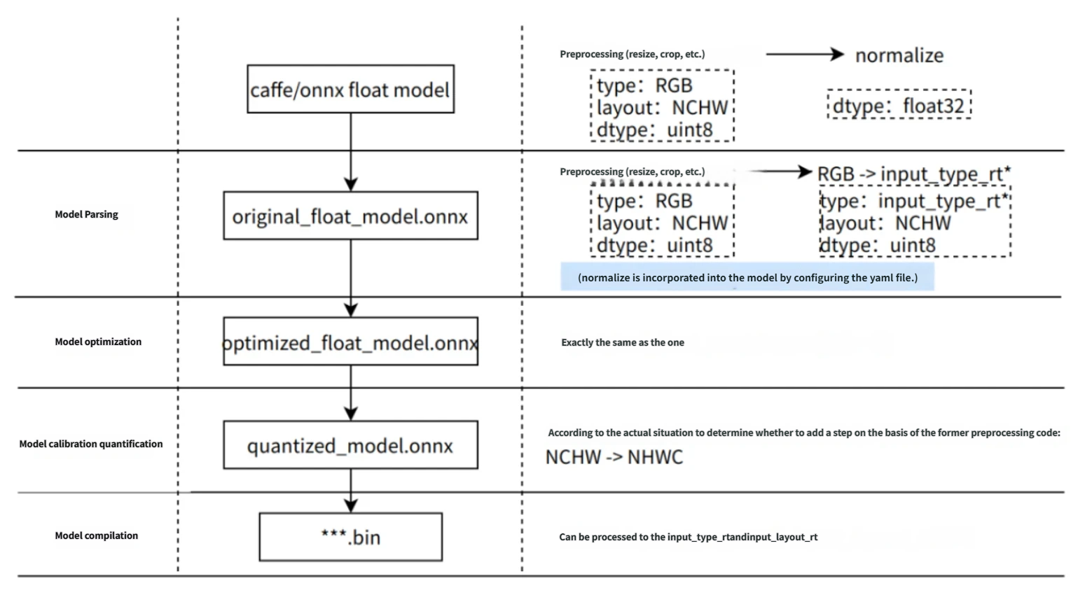
Remark:

input_type_rt* represents the intermediate format of input_type_rt.
Please use the visualization tool Netron to view the `quantized_model.onnxdata layout of the input nodes to decide whether to addlayout conversion`` to preprocessing.

Model analysis phaseFor Caffe floating point model, the conversion to the ONNX floating point model will be completed. On the original floating-point model, whether to join the data preprocessing node will be determined based on the configuration parameters in the transformation configuration yaml file. In this stage, an original_float_model.onnx is produced. The calculation accuracy of this ONNX model is still float32, but a data preprocessing node is added to the input part.

Ideally, this preprocessing node should complete the complete conversion of input_type_rt to input_type_train, The actual situation is that the entire type conversion process will be completed with the X5 processor hardware, and the ONNX model does not contain the hardware conversion part. Therefore, the real input type of ONNX will use an intermediate type, which is the hardware processing result type for input_type_rt. The data layout (NCHW/NHWC) will keep the input layout of the original floating point model consistent. Each type of input_type_rt has a specific corresponding intermediate type, as shown in the table:

nv12	yuv444	rgb	bgr	gray	featuremap
yuv444_128	yuv444_128	RGB_128	BGR_128	GRAY_128	featuremap

Remark:

The bold part of the first row in the table is the data type specified by input_type_rt, and the second row is the intermediate type corresponding to the specific input_type_rt. This intermediate type is the input type of original_float_model.onnx. Each type is explained as follows:

yuv444_128 is the result of yuv444 data minus 128, and each value is expressed by int8.
RGB_128 is the result of minus 128 of RGB data, and each value is expressed by int8.
BGR_128 is the result of minus 128 of BGR data, and each value is expressed by int8.
GRAY_128 is the result of minus 128 of gray data, and each value is expressed by int8.
featuremap is a four-dimensional tensor data, each value is represented by float32.

Model Optimization PhaseImplement some operator optimization strategies for the model that are suitable for the X5 platform, such as BN fusion to Conv, etc. The output of this stage is an optimized_float_model.onnx. The calculation accuracy of this ONNX model is still float32, and it will not affect the calculation results of the model after optimization. The input data requirements of the model are still consistent with the previous original_float_model.

Model Calibration PhaseThe calibration data you provide will be used to calculate the necessary quantization threshold parameters. These parameters will be entered directly into the quantization phase without generating a new model state. Model Quantization PhaseModel quantization is completed using the parameters obtained by calibration, and the output of this phase is a quantized_model.onnx. The calculation accuracy of this model is already int8. Using this model, you can evaluate the accuracy loss caused by model quantization. This model requires that the input basic data format and layout are still the same as original_float_model, but layout and numerical representation have changed. The overall changes compared to the original_float_model input are described as follows:

When the value of input_type_rt is not featuremap, all input data types are INT8. On the contrary, when the value of input_type_rt is featuremap, the input data type is float32.
The data layout layout relationship is: input_layout_train and the layout inputs of origin.onnx, calibrated_model.onnx, quanti.onnx are consistent with the layout inputs of the original model.

Notice: If input_type_rt is nv12, the corresponding input layout of quanti.onnx is NHWC.

Model compilation stageThe X5 algorithm toolchain model compiler will be used to convert the quantitative model into computing instructions and data supported by the X5 platform. At this stage, a ***.bin model is produced. This bin model is a model that can be run on the X5 embedded platform, which is the final output result of the model conversion.

Interpretation of conversion results

This section will introduce the interpretation of the successful state of the model conversion and the analysis method of unsuccessful conversion. To confirm that the model conversion is successful, you need to confirm from three aspects: makertbin status information, similarity information and working_dir output. In terms of status information, if the conversion is successful, a clear prompt message will be given at the end of the console output information as follows:

  2023-12-06 11:13:08,337 INFO Convert to runtime bin file successfully!
  2023-12-06 11:13:08,337 INFO End Model Convert

Similarity information also exists in the console output content of makertbin. Before the makertbin status information, its content form is as follows:

  ===============================================================================================
  Node ON Subgraph Type Cosine Similarity Threshold
  ... ... ... 0.999936 127.000000
  ... ... ... 0.999868 2.557209
  ... ... ... 0.999268 2.133924
  ... ... ... 0.996023 3.251645
... ... ... 0.996656 4.495638

Among the output content listed above:

The interpretations of Node, ON, Subgraph, Type and the hb_mapper checker tool are consistent. Please refer to the previous article Interpretation of Check Results;
Threshold is the calibration threshold for each level, which is used to feedback information to technical support in abnormal states, and does not require attention in normal conditions;
Cosine Similarity column reflects the cosine similarity between the original floating-point model of the corresponding operator in the Node column and the output results of the quantized model.

Tips:

In general, a model output node with Cosine Similarity >= 0.99 indicates normal quantization of the model. If the cosine similarity at the output node is below 0.8, noticeable accuracy degradation may occur. Note that Cosine Similarity is only a reference indicator for data stability after quantization and does not directly correlate with model accuracy.
For fully accurate accuracy assessment, please refer to the section Model Accuracy Analysis and Optimization.

The conversion outputs are stored in the path specified by the configuration parameter working_dir. After successful model conversion,
you will find the following files in that directory (where *** is the prefix specified via the configuration parameter output_model_file_prefix):

***_original_float_model.onnx
***_optimized_float_model.onnx
***_calibrated_model.onnx
***_quantized_model.onnx
***.bin

The section Interpretation of Conversion Outputs explains the purpose of each generated file.

Note:
Before deploying on hardware, we recommend completing the model performance & accuracy evaluation process introduced in Model Performance Analysis and Optimization to avoid extending model conversion issues into the embedded phase.

If any of the three aspects mentioned above for validating successful model conversion are missing, it indicates an error occurred during conversion.
In most cases, the makertbin tool will output error messages to the console when an error occurs.
For example, if during Caffe model conversion the prototxt and caffe_model parameters in the YAML file are not configured, the model conversion tool will produce the following prompt:

2021-04-21 14:45:34,085 ERROR Key 'model_parameters' error:
Missing keys: 'caffe_model', 'prototxt'
2021-04-21 14:45:34,085 ERROR yaml file parse failed. Please double check your input
2021-04-21 14:45:34,085 ERROR exception in command: makertbin

If console logs do not help identify the issue, please refer to the Algorithm Toolchain - Common Troubleshooting section for further investigation. If the issue remains unresolved, please contact technical support or post your question on the Official Technical Community. We will provide assistance within 24 hours.

Interpretation of Conversion Outputs

As mentioned above, successful model conversion generates the following five files. This section explains the purpose of each:

***_original_float_model.onnx
***_optimized_float_model.onnx
***_calibrated_model.onnx
***_quantized_model.onnx
***.bin

The generation process of ***_original_float_model.onnx is described in Interpretation of Internal Conversion Process.
This model has the same computational accuracy as the original floating-point model provided as input. A key difference is that preprocessing operations have been added to adapt to the X5 platform (an additional preprocessing operator node HzPreprocess is added; you can view this using tools like Netron. For details about this operator, see HzPreprocess Operator Description).
Generally, you do not need to use this model. However, if issues persist after applying the troubleshooting methods described earlier, providing this model to technical support or posting your issue on the Official Technical Community can help resolve the problem more quickly.

The generation process of ***_calibrated_model.onnx is described in Interpretation of Internal Conversion Process.
This model is an intermediate product generated after the model conversion toolchain optimizes the structure of the floating-point model and computes quantization parameters for each node using calibration data, which are then stored in calibration nodes.

The generation process of ***_optimized_float_model.onnx is described in Interpretation of Internal Conversion Process.
This model has undergone operator-level optimizations, such as operator fusion.
By visually comparing it with the original_float model, you can clearly observe structural changes at the operator level, though these do not affect computational accuracy.
Generally, you do not need to use this model. However, if issues persist after applying the troubleshooting methods described earlier, providing this model to technical support or posting your issue on the Official Technical Community can help resolve the problem more quickly.

The generation process of ***_quantized_model.onnx is described in Interpretation of Internal Conversion Process.
This model has completed the calibration and quantization process. To evaluate accuracy loss after quantization, please read the Model Accuracy Analysis and Optimization section below.
This model must be used during accuracy validation. For specific usage instructions, refer to Model Accuracy Analysis and Optimization.

***.bin is the model file ready to be loaded and executed on the X5 processor.
Combined with the content introduced in the “Runtime Application Development Guide” section,
you can quickly deploy and run the model on the X5 processor. However, to ensure the model’s performance and accuracy meet your expectations,
we recommend completing the performance and accuracy analysis processes described in Model Conversion and Model Accuracy Analysis and Optimization before proceeding to application development and deployment.

Note:

Typically, you can obtain a model ready to run on the X5 processor after completing the model conversion phase. However, to ensure the model’s performance and accuracy meet application requirements, we recommend performing subsequent performance and accuracy evaluation steps after each conversion.

The model conversion process generates ONNX models, which are intermediate artifacts intended to help users verify model accuracy. Therefore, backward compatibility across versions is not guaranteed. When using evaluation scripts from examples to evaluate ONNX models (either on single images or test sets), please regenerate the ONNX models using the current version of the tool.

6.3.2.5. Model Performance Analysis

This section introduces how to use tools provided by the X5 algorithm toolchain to evaluate model performance. These tools yield performance results closely matching actual hardware execution. If evaluation results do not meet expectations, we recommend following the optimization suggestions provided by the X5 algorithm toolchain to resolve performance issues before entering the application development phase.

Performance Evaluation on Development Machine

Use the hb_perf tool to evaluate model performance. Usage:

  hb_perf  ***.bin

Note:
If analyzing a packed model, add the -p parameter: hb_perf -p ***.bin.
For more information about model pack, see the “Other Model Tools (Optional)” section.

The ***.bin in the command refers to the fixed-point model generated during the model conversion step. After execution, a folder named hb_perf_result is created in the current directory, containing detailed model analysis results.
Below is an example result for the MobileNetv1 model:

  hb_perf_result/
  └── mobilenetv1_224x224_nv12
      ├── MOBILENET_subgraph_0.html
      ├── MOBILENET_subgraph_0.json
      ├── mobilenetv1_224x224_nv12
      ├── mobilenetv1_224x224_nv12.html
      ├── mobilenetv1_224x224_nv12.png
      └── temp.hbm

Open mobilenetv1_224x224_nv12.html in a browser. The content appears as follows:

hb_mapper_perf_2

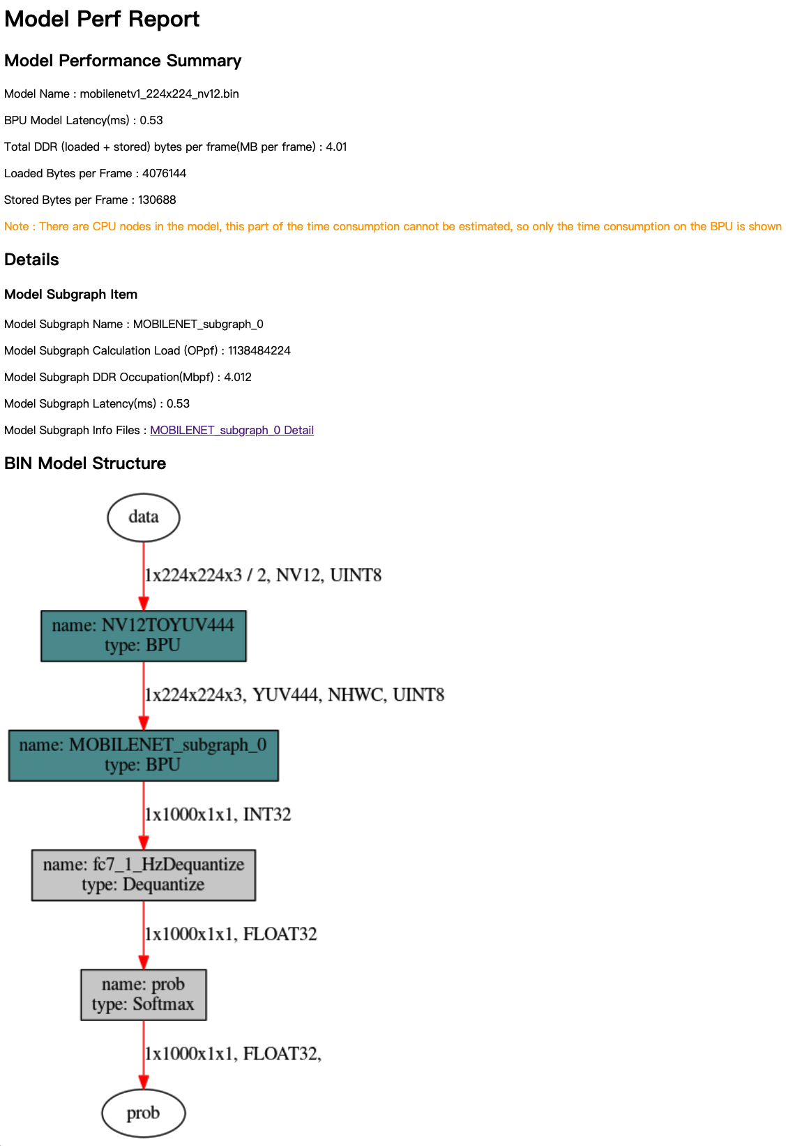
The analysis results consist of three main parts: Model Performance Summary, Details, and BIN Model Structure.
Model Performance Summary provides an overall performance evaluation of the bin model, with the following metrics:

Model Name — Name of the model.
Model Latency(ms) — End-to-end inference latency per frame (in milliseconds).
Total DDR (loaded+stored) bytes per frame(MB per frame) — Total DDR usage per frame for BPU data loading and storage (in MB/frame).
Loaded Bytes per Frame — Data read per frame during model execution.
Stored Bytes per Frame — Data written per frame during model execution.

The BIN Model Structure section provides a subgraph-level visualization of the bin model. Dark cyan nodes represent operations running on the BPU, while gray nodes represent CPU computations.

When reviewing Details and BIN Model Structure, you should understand the concept of subgraphs.
If the model contains operators designated for CPU execution, the model conversion tool splits the BPU-computable segments before and after the CPU operator into two independent subgraphs.
For more details, refer to the Model Validation section.

Details provide specific information for each BPU subgraph of the model. In the mobilenetv1_224x224_nv12.html main page, the metrics for each subgraph include:

Model Subgraph Name — Name of the subgraph.
Model Subgraph Calculation Load (OPpf) — Computation load per frame.
Model Subgraph DDR Occupation(Mbpf) — Data read/write volume per frame (in MB).
Model Subgraph Latency(ms) — Inference latency per frame (in ms).

Each subgraph result includes detailed reference information.

Note:

The reference information page varies depending on whether debugging configuration (debug) is enabled.
The Layer Details shown in the figure below are only available when the debug parameter in the YAML configuration file is set to True.
For instructions on configuring the debug parameter, refer to Model Conversion YAML Configuration Parameters.

Layer Details provide operator-level analysis and can be used as a reference during model debugging and analysis. For example, if certain BPU operators cause poor performance, the analysis results can help pinpoint the specific operators.

layer_details

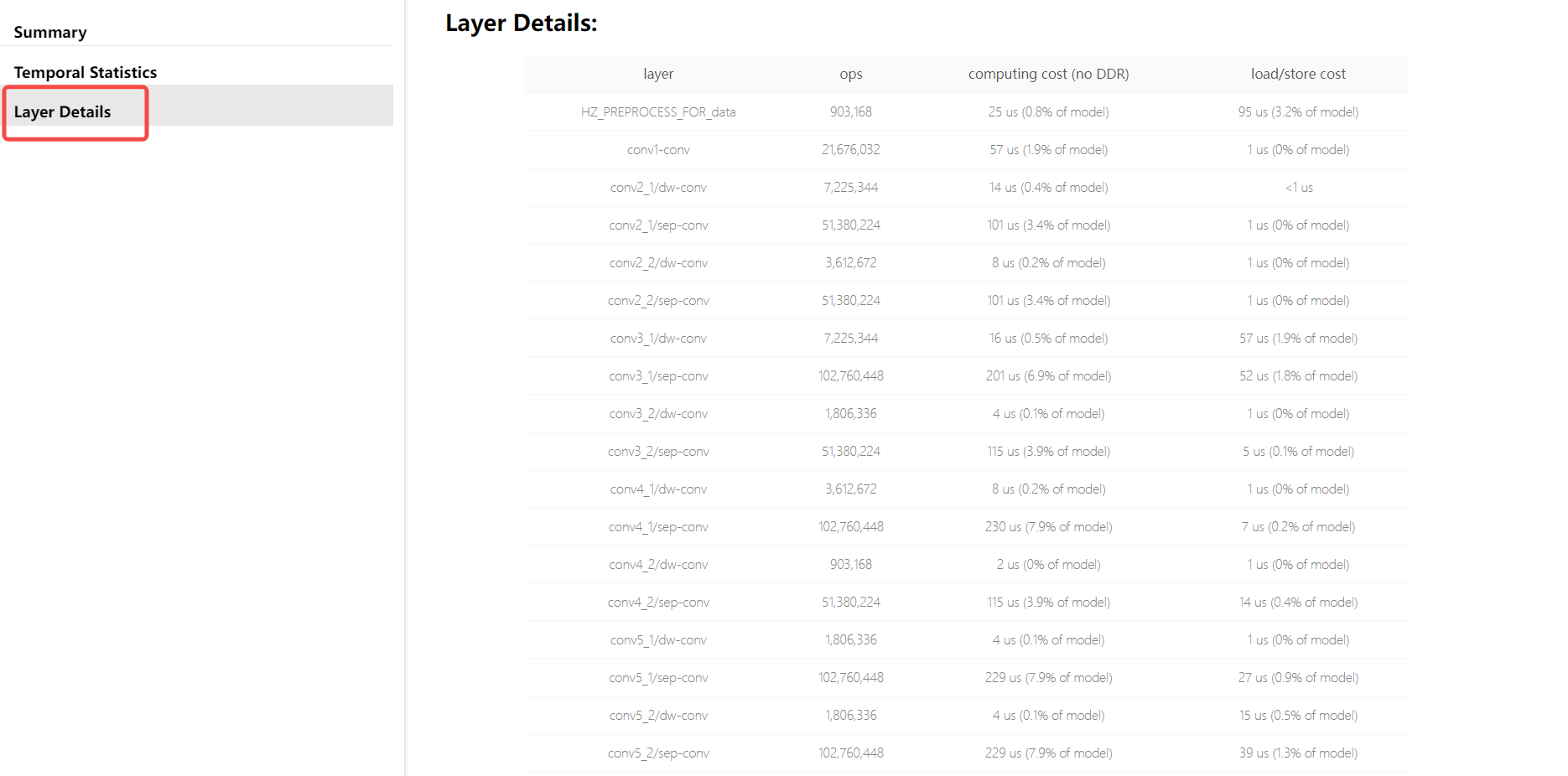
Each metric is interpreted as follows:

layer — Name of the layer.
ops — Computation load.
original output shape — Original operator output shape.
aligned output shape — Aligned operator output shape.
computing cost (no DDR) — Computation time.
load/store cost — Data transfer time.
active period of time — Active time period of the layer after compilation (does not represent actual execution time, often involving alternating/parallel execution of multiple layers).

Note:
The results from the hb_perf tool help you understand the subgraph structure of the bin model and provide static analysis metrics for BPU computation parts. Note that the analysis results do not include CPU computation evaluation. For CPU performance, conduct real-world measurements on the development board.

Performance Measurement on Development Board

To quickly evaluate model performance on the development board, use the hrt_model_exec perf tool, which directly measures inference performance and retrieves model information on the board.

Before using the hrt_model_exec perf tool, prepare the following:

Ensure you have completed the system update on the development board as described in the system update section.
Copy the bin model generated on the Ubuntu development machine to the development board (recommended to place in the /userdata directory).
Since the development board runs a Linux system, you can use common Linux methods like scp to perform this copy.

The command for hrt_model_exec perf is as follows (note: execute on the development board):

./hrt_model_exec perf --model_file mobilenetv1_224x224_nv12.bin \
                      --model_name="" \
                      --core_id=0 \
                      --frame_count=200 \
                      --perf_time=0 \
                      --thread_num=1 \
                      --profile_path="."

Explanation of hrt_model_exec perf parameters:

model_file:
Name of the bin model to analyze.

model_name:
Name of the bin model to analyze. Can be omitted if model_file contains only one model.

core_id:
Default value 0. Core ID used to run the model.

frame_count:
Default value 200. Number of inference frames. The tool runs the specified number of inferences and calculates average latency. Effective when perf_time is 0.

perf_time:
Default value 0, unit in minutes. Inference duration. The tool runs for the specified time and calculates average latency.

thread_num:
Default value 1, range [1,8]. Number of threads. To analyze peak frame rate, increase the thread count.

profile_path:
Disabled by default. Specifies the path for logging profiler data. Results will be saved in profiler.log and profiler.csv files under the specified directory.

The following example shows test results on an X5 development board. After command execution, you will see logs like this on the console:

  Running condition:
    Thread number is: 4
    Frame count   is: 1000
    Program run time: 279.004000 ms
  Perf result:
    Frame totally latency is: 1084.040527 ms
    Average    latency    is: 1.084041 ms
    Frame      rate       is: 3584.178005 FPS

Tips:
In the evaluation results, Average latency and Frame rate represent average per-frame inference latency and model peak frame rate, respectively.
To obtain the model’s peak frame rate on the board, try adjusting the thread_num value to find the optimal number of threads, as different values yield different performance results.

Console output only shows overall results. By setting the profile_path parameter, the generated node_profiler.log file records richer model performance information:

{
    "perf_result": {
      "FPS": 3718.384436330103,
      "average_latency": 1.0366870164871216
    },
    "running_condition": {
      "core_id": 0,
      "frame_count": 1000,
      "model_name": "mobilenetv1_224x224_nv12",
      "run_time": 268.934,
      "thread_num": 4
    }
  }
  ***
  {
    "processor_latency": {
      "BPU_inference_time_cost": {
        "avg_time": 0.8493590000000001,
        "max_time": 1.328,
        "min_time": 0.766
      },
      "CPU_inference_time_cost": {
        "avg_time": 0.074976,
        "max_time": 0.382,
        "min_time": 0.066
      }
    },
    "model_latency": {
      "BPU_MOBILENET_subgraph_0": {
        "avg_time": 0.8493590000000001,
        "max_time": 1.328,
        "min_time": 0.766
      },
      "Dequantize_fc7_1_HzDequantize": {
        "avg_time": 0.029727,
        "max_time": 0.124,
        "min_time": 0.028
      },
      "MOBILENET_subgraph_0_output_layout_convert": {
        "avg_time": 0.011379,
        "max_time": 0.077,
        "min_time": 0.008
      },
      "Preprocess": {
        "avg_time": 0.005363000000000001,
        "max_time": 0.039,
        "min_time": 0.003
      },
      "Softmax_prob": {
        "avg_time": 0.028507,
        "max_time": 0.142,
        "min_time": 0.027
      }
    },
    "task_latency": {
      "TaskPendingTime": {
        "avg_time": 0.021235,
        "max_time": 0.336,
        "min_time": 0.002
      },
      "TaskRunningTime": {
        "avg_time": 0.983558,
        "max_time": 2.208,
        "min_time": 0.904
      }
    }
  }

The above log corresponds to the BIN Model Structure section described in Performance Estimation Using hb_perf Tool.
Each node in the visualization has a corresponding entry in the profiler.log file, identifiable by name. Additionally, the profiler.log file records execution times for each node, providing references for optimizing model operators. Since BPU nodes have special requirements for input/output (e.g., specific layout and padding alignment), preprocessing of input and output data is required.

Preprocess: Represents padding and layout conversion operations on model input data; timing is recorded under Preprocess.
xxxx_input_layout_convert: Represents padding and layout conversion on BPU node input data; timing is recorded under xxxx_input_layout_convert.
xxxx_output_layout_convert: Represents removal of padding and layout conversion on BPU node output data; timing is recorded under xxxx_output_layout_convert.

profiler analysis is a common operation in model performance optimization. As mentioned in the previous section Interpretation of Validation Results, CPU operators may not require much attention during validation, but in this stage, you can see their actual execution time, enabling performance tuning based on per-operator timing.

Model Performance Optimization

Based on the above performance analysis results, you may find the model performance below expectations. This section provides recommendations and measures to improve model performance, including checking YAML configuration parameters, handling CPU operators, high-performance model design suggestions, and using X5-platform-friendly structures and models.

Note:
Some modification suggestions in this section may affect the parameter space of the original floating-point model, requiring retraining. To avoid repeated adjustments and retraining during performance optimization, we recommend using randomly initialized parameters to export and validate performance before achieving satisfactory model performance.

Check YAML Parameters Affecting Model Performance

In the YAML configuration file for model conversion, certain parameters directly affect the final model performance. Please first verify they are correctly configured as expected.
For detailed meanings and functions of each parameter, refer to the Compiler Parameters Group section.

layer_out_dump: Specifies whether to output intermediate results during model conversion, typically used only for debugging.
If set to True, a dequantization output node is added for each convolution operator, significantly degrading on-board model performance.
Therefore, during performance evaluation, ensure this parameter is set to False.
compile_mode: Used to select whether model compilation optimizes for bandwidth or latency. Set to latency when prioritizing performance.
optimize_level: Used to select the compiler optimization level. For best performance, set to O3 in practice.
debug: Setting to True enables compiler debug mode, outputting performance simulation information such as frame rate and DDR bandwidth usage. Useful during performance evaluation; can be disabled before product delivery to reduce model size and improve execution efficiency.
max_time_per_fc: Controls the execution duration of function calls for compiled model data instructions, enabling model priority preemption.
Changing this parameter to adjust the execution duration of preempted models affects on-board model performance.

Handling CPU Operators

Based on evaluation using the hrt_model_exec perf tool, if you confirm that model performance bottlenecks are caused by CPU operators, we recommend checking the Model Operator Support List to determine whether the currently CPU-running operators have BPU support.

If the operator is listed as BPU-supported, the issue likely stems from operator parameters exceeding BPU-supported constraints. We recommend adjusting the corresponding original floating-point model parameters within the supported range.
To quickly identify which specific parameters exceed constraints, we suggest re-running the validation method described in the Model Validation section, which will directly highlight parameters beyond BPU support limits.

Note:
You are responsible for assessing the impact of modifying original floating-point model parameters on accuracy. For example, exceeding input_channel or output_channel limits in Convolution is a typical case. Reducing channels may enable BPU support but could also affect model accuracy.

If the operator lacks BPU support, apply the following optimizations accordingly:

CPU operator located in the middle of the model

For CPU operators in the middle of the model, we recommend first attempting parameter adjustment, operator replacement, or model modification.
CPU operator located at the beginning or end of the model

For CPU operators at the beginning or end of the model, refer to the following examples. Take quantization/dequantization nodes as examples:
- For nodes connected to model input/output, add the remove_node_type parameter in the model_parameters configuration group of the YAML file and recompile the model.
```
  remove_node_type: "Quantize; Dequantize"
```
  Or use the hb_model_modifier tool to modify the bin model:
```
  hb_model_modifier x.bin -a Quantize -a Dequantize
```
- For models like the one below where nodes are not directly connected to input/output, use the hb_model_modifier tool to check whether connected nodes can be removed and delete them sequentially.
  
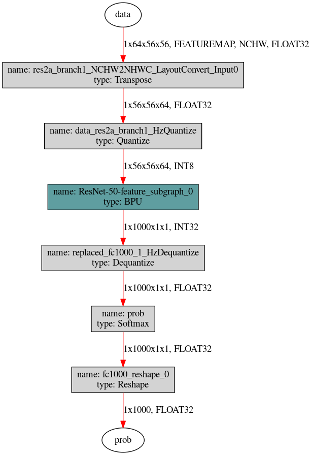
  First use the hb_perf tool to get the model structure diagram, then use the following two commands to remove the Quantize node top-down.
  For Dequantize nodes, remove them bottom-up. The names of removable nodes at each step can be viewed via hb_model_modifier x.bin.
```
  hb_model_modifier x.bin -r res2a_branch1_NCHW2NHWC_LayoutConvert_Input0
  hb_model_modifier x_modified.bin -r data_res2a_branch1_HzQuantize
```

High-Performance Model Design Recommendations

Based on performance evaluation results, if CPU computation time percentage is very small, the performance bottleneck is likely due to excessive BPU inference time.
This indicates the model has already utilized all available BPU computing units, so the next step is to improve computational resource utilization.
Since each processor has unique hardware characteristics, whether the model’s computational parameters align well with these characteristics directly determines computational resource utilization—better alignment leads to higher utilization, and vice versa.

This section focuses on the hardware characteristics of the X5 processor: it is designed to accelerate CNN (Convolutional Neural Networks), with most computational resources dedicated to various convolution operations. We recommend using models primarily based on convolution operations, as non-convolution operators reduce computational resource utilization, with varying degrees of performance impact.
Additionally, during model design, try to minimize the input and output dimensions of BPU segments to reduce quantization/dequantization node overhead and hardware bandwidth pressure.
Taking a typical segmentation model as an example, you can directly incorporate the Argmax operator into the model itself. However, note that Argmax supports BPU acceleration only under the following conditions:

In Caffe, Softmax layer defaults to axis=1, while ArgMax layer defaults to axis=0. Consistency in axis must be maintained during operator replacement.
Argmax’s Channel must be ≤ 64; otherwise, it can only be computed on the CPU.

6.3.2.6. Model Accuracy Analysis

Post-training quantization (PTQ), which converts floating-point models to fixed-point models using dozens or hundreds of calibration data samples, inevitably incurs some accuracy loss.
The PTQ conversion tool in the X5 algorithm toolchain, validated through extensive real-world usage, typically keeps model accuracy loss within 1% by selecting optimal quantization parameter combinations in most cases.

This section first explains how to correctly perform model accuracy analysis. If evaluation results are unsatisfactory, you can refer to the Accuracy Optimization subsection for model accuracy tuning.

Accuracy Analysis

As mentioned earlier, successful model conversion generates the following files:

***_original_float_model.onnx
***_optimized_float_model.onnx
***_calibrated_model.onnx
***_quantized_model.onnx
***.bin

Although the final bin model is the one deployed on the X5 processor, to facilitate quick accuracy testing on Ubuntu/CentOS development machines, we also support using ***_quantized_model.onnx for model accuracy testing. The quantized model has consistent accuracy with the bin model running on the X5 processor.

We recommend using the X5 SDK to load the ONNX model for inference. The basic process is as follows:

Note:

The example code applies not only to quantized models but also to original and optimized models. Prepare data according to the input type and layout requirements of different models for inference.
We recommend referring to the accuracy validation methods for example models (Caffe, ONNX, etc.) in the horizon_model_convert_sample example package of the X5 algorithm toolchain: 04_inference.sh and postprocess.py.

import numpy as np
# Load D-Robotics dependency library
from horizon_tc_ui import HB_ONNXRuntime

# Prepare model input
input_data = np.load("input.npy")
# Load model file
sess = HB_ONNXRuntime(model_file = "***_quantized_model.onnx")
# Get model input & output node information
input_names = sess.input_names
output_names = sess.output_names
# Prepare input data (assuming the model has only one input)
input_info = {input_names[0]: input_data}
# Start inference; output is a list corresponding to output_names
output = sess.run(output_names, input_info)

Additionally, input data preparation is the most error-prone step. Compared to the accuracy validation process during original floating-point model design & training, we recommend adjusting the inference input data after preprocessing: mainly data format (RGB, NV12, etc.), data precision (int8, float32, etc.), and data layout (NCHW or NHWC).
The adjustment method is determined by the four parameters input_type_train, input_layout_train, input_type_rt, and input_layout_rt set in the YAML configuration file during model conversion. For detailed rules, refer to the Interpretation of Internal Conversion Process section.

For example, consider an original floating-point classification model trained on ImageNet with a single input node accepting three-channel images in BGR order with NCHW layout.
During the original floating-point model design & training phase, the data preprocessing before inference on the validation set includes:

Resize image proportionally so the shorter side is 256.
Use center_crop to obtain a 224x224 image.
Subtract mean per channel.
Multiply data by scale factor.

When converting this original floating-point model using the X5 algorithm toolchain,
set input_type_train to bgr, input_layout_train to NCHW, input_type_rt to bgr,
and input_layout_rt to NHWC.
According to the rules described in Interpretation of Internal Conversion Process, ***_quantized_model.onnx expects input in bgr_128 format with NHWC layout.
Corresponding to the example code above, the data preparation process in your_custom_data_prepare should be:

  # This example uses skimage; OpenCV would differ
  # Note: Transformers do not include mean subtraction or scaling
  # Mean and scale operations are fused into the model; see norm_type/mean_value/scale_value configuration earlier
def your_custom_data_prepare_sample(image_file):
    # skimage reads image in NHWC layout
    image = skimage.img_as_float(skimage.io.imread(image_file))
    # Resize proportionally, short side to 256
    image = ShortSideResize(image, short_size=256)
    # CenterCrop to 224x224
    image = CenterCrop(image, crop_size=224)
    # skimage reads RGB; convert to BGR for bgr_128
    image = RGB2BGR(image)
    # If original model uses NCHW input (except when input_type_rt is nv12)
    if layout == "NCHW":
      image = HWC2CHW(image)
    # skimage values in [0.0,1.0]; scale to bgr range
    image = image * 255
    # bgr_128 is bgr minus 128
    image = image - 128
    # bgr_128 uses int8
    image = image.astype(np.int8)
    
    return image

Accuracy Optimization

Based on the accuracy analysis above, if quantization accuracy does not meet expectations, resolve according to the following two scenarios:

Significant accuracy loss (greater than 4%).
This is often caused by improper YAML configuration or imbalanced calibration datasets. We recommend checking the suggestions below one by one.
Minor accuracy loss (1.5%~3%).
After ruling out issues from case 1, if there is still minor accuracy degradation, it is likely due to model sensitivity. We recommend using the accuracy optimization tools provided by the X5 algorithm toolchain.
If accuracy remains unsatisfactory after trying cases 1 and 2, try using our provided accuracy debug tools for further investigation.

The overall accuracy issue resolution process is illustrated below:

accuracy_problem

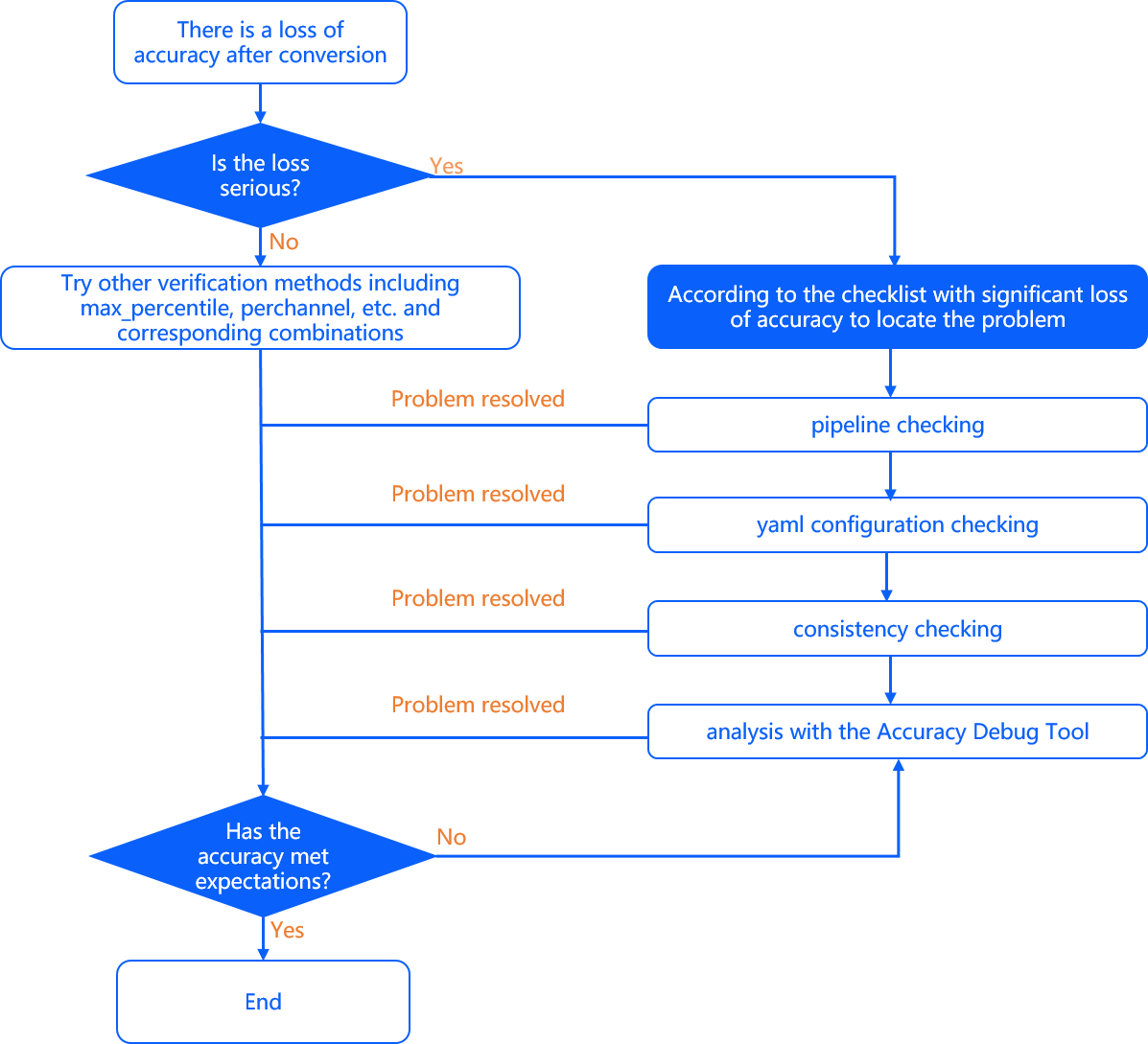
Significant Accuracy Loss (Over 4%)

If the model accuracy loss exceeds 4%, it is typically caused by improper YAML configuration, imbalanced validation datasets, etc. It is recommended to troubleshoot step by step from the following aspects: pipeline, model conversion configuration, and consistency checks.

Pipeline Inspection:

The pipeline refers to your complete process of data preprocessing, model conversion, model inference, post-processing, and accuracy evaluation. Please verify each of these steps according to the corresponding sections above.
Based on past issue-tracking experiences, we find that in most cases, changes made during the original floating-point model training phase were not timely reflected in the model conversion step, leading to abnormal accuracy validation results.

Model Conversion YAML Configuration Check:

According to the recommended workflow for PTQ accuracy evaluation and consistency verification, if the accuracy issue is traced back to original_float.onnx, we recommend carefully reviewing the YAML configuration file and preprocessing/postprocessing code for errors. Common pitfalls in the YAML configuration include:

input_type_rt and input_type_train: These parameters differentiate the data format required by the mixed heterogeneous model after conversion and the original floating-point model. Ensure they are correctly set, especially regarding BGR and RGB channel order.
Correctness of parameters such as norm_type, mean_value, and scale_value. These configurations can directly insert mean and scale operation nodes into the model. Confirm whether the validation/test images undergo duplicate mean and scale operations—repeated preprocessing is a common source of errors.

Data Processing Consistency Check:

Incorrectly specifying read_mode: In 02_preprocess.sh, the image reading mode can be set via the --read_mode parameter, supporting opencv and skimage.
Additionally, preprocess.py also sets the image reading mode via the imread_mode parameter, which should be modified accordingly. Using skimage for image loading results in RGB channel order, value range 0~1, and data type float; whereas using opencv yields BGR channel order, value range 0~255, and data type uint8.
Incorrect storage format of calibration dataset: Currently, X5 uses numpy.tofile to save calibration data, which does not preserve shape or data type information. During loading, these must be manually specified. Ensure consistency in data type, dimensions, and layout during serialization and deserialization. If input_type_train is in non-featuremap format, the data dtype is determined by whether the calibration data path contains “f32”: if so, data is parsed as float32; otherwise, as uint8.
Inconsistency in transformer implementation: We provide a series of common preprocessing functions located in /horizon_model_convert_sample/01_common/python/data/transformer.py. Implementation differences in certain preprocessing operations may exist. For example, ResizeTransformer uses OpenCV’s default interpolation method (linear). If a different interpolation method is used, modify the source code in transformer.py to ensure consistency with the training preprocessing code. Refer to the transformer usage guide section for details.
During the X5 algorithm toolchain usage, continue using the same data processing libraries relied upon during original floating-point model training and validation.
For models with poor robustness, differences in implementations of typical operations (e.g., resize, crop) across libraries may introduce disturbances that affect model accuracy.
Proper setup of the validation image set: The calibration dataset should contain approximately one hundred images, ideally covering various data distribution scenarios. For multi-task or multi-class models, ensure the validation set covers all prediction branches or categories.
Avoid anomalous images that deviate from the data distribution (e.g., overexposed images).
Re-validate accuracy using ***_original_float_model.onnx. Under normal circumstances, the accuracy of this model should align with the original floating-point model up to three to five decimal places.
If this level of alignment is not achieved, further inspect your data processing pipeline.

Minor Accuracy Loss Optimization (1.5%~3%)

Generally, to reduce the difficulty of accuracy tuning, we recommend first trying to set calibration_type to default. The default option enables an automatic search feature that selects the optimal calibration method (from max, max-Percentile 0.99995, and KL) based on the cosine similarity of the output node from the first calibration sample.
The selected calibration method can be found in the conversion log, e.g., a message like “Select kl method.”. During the search, the tool also evaluates options such as per-channel quantization and asymmetric (Asymmetric) quantization.

If per-channel quantization is enabled, the log will print: Perchannel quantization is enabled.
If asymmetric quantization is enabled, the log will print: Asymmetric quantization is enabled.

If the automatically selected calibration method still results in accuracy loss between 1.5% and 3% compared to the original floating-point model, consider the following optimization suggestions:

Adjust Calibration Method:

Manually specify calibration_type in the configuration. Start with mix; if accuracy remains unsatisfactory, try kl or max.
When calibration_type is set to max, configure max_percentile to different percentiles (range: 0.5–1). We recommend trying 0.99999, 0.99995, 0.9999, 0.9995, and 0.999. Observe the trend in model accuracy across these settings to find the optimal percentile.
Based on the above trials, select the configuration with the highest cosine similarity and try enabling per_channel in the conversion configuration.
The optimization parameter in the YAML file provides options asymmetric and bias_correction for accuracy debugging. Experiments show these can improve quantization accuracy in certain scenarios—further experimentation is encouraged.

Refine Calibration Dataset:

Try appropriately increasing or decreasing the number of calibration samples (typically, detection tasks require fewer calibration samples than classification tasks). Also, observe model output for missed detections and increase calibration data for corresponding scenarios.
Observe model output for missed detections and add more calibration data for those specific scenarios.
Avoid pure black/white or other anomalous data. Minimize using background images without targets. Ensure comprehensive coverage of typical task scenarios so that the calibration dataset distribution closely matches the training set.

Revert part Tail Operators to High-Precision CPU Computation:

Generally, only attempt to revert 1～2 operators near the model output layer to CPU. Too many CPU operators significantly impact overall model performance. The decision can be based on observing the model’s cosine similarity—if moving certain intermediate nodes to CPU does not improve accuracy, this is normal, as repeated re-quantization may introduce greater accuracy loss. Therefore, only tail nodes are typically recommended for CPU fallback.
Specify operators to run on CPU via the node_info parameter in the YAML file.

Accuracy Debug Tool

After trying the above two accuracy optimization methods, if accuracy still does not meet expectations, you may use our accuracy debug tool.
During the PTQ post-quantization process, accuracy loss mainly stems from two causes: sensitive node quantization issues and accumulated quantization error across nodes.
To help you locate these issues, we provide an accuracy debug tool to assist in autonomously identifying accuracy problems during model quantization.
This tool enables node-level quantization error analysis on the calibrated model, helping you quickly identify nodes with abnormal accuracy degradation.

If you are using the X5 product, you may also try configuring certain ops to compute in int16 for accuracy tuning:

During model conversion, most ops default to int8 computation. In some scenarios, using int8 for certain ops may lead to significant accuracy loss.
For the X5 product, the current algorithm toolchain supports specifying certain ops to compute in int16. For details, refer to the int16 configuration guide.
By configuring accuracy-sensitive ops (based on cosine similarity) to compute in int16, accuracy loss can be mitigated in certain scenarios.

The algorithm toolchain calibrates and quantizes the model using your provided calibration samples to ensure efficient deployment on the X5 computing platform. However, during the conversion process, accuracy loss is inevitably introduced due to the transition from floating-point to fixed-point arithmetic. The main reasons for accuracy loss typically include:

Certain nodes in the model are highly sensitive to quantization, introducing large errors—this is known as the sensitive node quantization issue.
Accumulated errors across nodes lead to significant overall calibration error, including: accumulated error from weight quantization, activation quantization, and full-model quantization.

To address this, the X5 algorithm toolchain provides an accuracy debug tool to help you autonomously locate accuracy issues during model quantization.
This tool enables node-level quantization error analysis on the calibrated model, helping you quickly identify nodes with abnormal accuracy.

The accuracy debug tool offers multiple analysis functions, such as:

Obtaining node quantization sensitivity.
Obtaining the model’s cumulative error curve.
Obtaining data distribution for specified nodes.
Obtaining box plots of inter-channel data distribution for specified node inputs.

Usage Instructions

Using the accuracy debug tool involves the following steps:

In the YAML model_parameters section, configure debug_mode="dump_calibration_data" to save calibration data.
Import the debug module and load the calibrated model and data.
Use the API or command-line interface provided by the accuracy debug tool to analyze models with significant accuracy loss.

Note:

For the current version of the accuracy debug tool: X5 corresponds to the bayes-e architecture model, supporting both command-line and API usage.

The overall process is illustrated below:

accuracy_debug_process

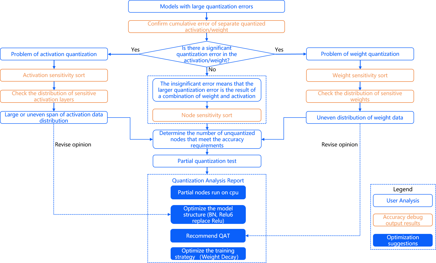
To check cumulative error for activation/weight quantization separately, refer to the plot_acc_error section.
For activation sensitivity ranking, refer to get_sensitivity_of_nodes.
For weight sensitivity ranking, refer to get_sensitivity_of_nodes.
For node sensitivity ranking, refer to get_sensitivity_of_nodes.
To view sensitive activation layer distributions, refer to plot_distribution and get_channelwise_data_distribution.
To view sensitive weight distributions, refer to plot_distribution and get_channelwise_data_distribution.
For sensitivity analysis via individual or partial node quantization, refer to sensitivity_analysis.

Saving Calibrated Model and Data:

First, configure debug_mode="dump_calibration_data" in the YAML file to enable accuracy debugging and save calibration data (calibration_data). The calibrated model (calibrated_model.onnx) is saved by default. Specifically:

Calibration data (calibration_data): During calibration, the model performs forward inference on these data to obtain quantization parameters (scale and threshold) for each quantized node.
Calibrated model (calibrated_model.onnx): Quantization parameters computed during calibration are saved in calibration nodes, resulting in the calibrated model.

Note:

What is the difference between the calibration data saved here and that generated by 02_preprocess.sh?

The calibration data from 02_preprocess.sh is in BGR color space. Internally, the toolchain converts it to the actual model input format (e.g., YUV444/gray).
The calibration data saved here, however, is in .npy format after color space conversion and preprocessing, and can be directly loaded via np.load() for model inference.

Note:

Understanding the Calibrated Model (calibrated_model.onnx)

The calibrated model is an intermediate artifact produced by the model conversion toolchain after structural optimization of the floating-point model and computation of quantization parameters for each node using calibration data.
Its key feature is the presence of calibration nodes of type HzCalibration, which fall into two categories: activation calibration nodes and weight calibration nodes.

Activation calibration nodes: Their input is the output of the preceding node. They quantize and dequantize the input using stored quantization parameters (scales and thresholds) before outputting.
Weight calibration nodes: Their input is the original floating-point weights. They quantize and dequantize the weights using stored quantization parameters before outputting.

Other nodes in the calibrated model are referred to by the accuracy debug tool as ordinary nodes (node), including types such as Conv, Mul, Add, etc.

debug_node

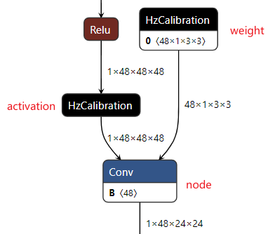
The folder structure of calibration_data is as follows:

|--calibration_data : calibration data
|----input.1 : folder named after model input node, containing corresponding input data
|--------0.npy
|--------1.npy
|-------- ...
|----input.2 : multiple folders for multi-input models
|--------0.npy
|--------1.npy
|-------- ...

Importing and Using the Debug Module

Next, import the debug module in your code and use the get_sensitivity_of_nodes interface to obtain node quantization sensitivity (default metric: cosine similarity of model output).
For detailed parameter descriptions of get_sensitivity_of_nodes, refer to the get_sensitivity_of_nodes section.

# Import debug module
import horizon_nn.quantizer.debugger as dbg
# Import logging module
import logging

# If verbose=True, set log level to INFO
logging.getLogger().setLevel(logging.INFO)
# Get node quantization sensitivity
node_message = dbg.get_sensitivity_of_nodes(
        model_or_file='./calibrated_model.onnx',
        metrics=['cosine-similarity', 'mse'],
        calibrated_data='./calibration_data/',
        output_node=None,
        node_type='node',
        data_num=None,
        verbose=True,
        interested_nodes=None)

Analysis Result Display

Below is the printed output when verbose=True:

=================node sensitivity=================
node                  cosine-similarity  mse
---------------------------------------------------
Conv_60               0.77795            68.02103
Conv_48               0.78428            64.36318
Conv_82               0.80394            61.09268
Conv_94               0.80499            65.05224
Conv_42               0.83787            49.4949
Conv_88               0.84614            49.81132
Conv_54               0.86602            41.69972
Conv_71               0.87148            39.96296
Conv_65               0.87495            40.45997
Conv_25               0.89214            34.30351
Conv_20               0.89829            32.35053
Conv_77               0.89916            31.9907
Conv_14               0.90058            32.40179
Conv_9                0.90107            34.08191
Conv_37               0.91162            28.21194
Conv_31               0.91637            28.79291

Additionally, this API returns the node sensitivity information as a dictionary (Dict) for further analysis.

Out:
{'Conv_60': {'cosine-similarity': 0.77795, 'mse': 68.02103},
 'Conv_48': {'cosine-similarity': 0.78428, 'mse': 64.36318},
 'Conv_82': {'cosine-similarity': 0.80394, 'mse': 61.09268},
 'Conv_94': {'cosine-similarity': 0.80499, 'mse': 65.05224},
 'Conv_42': {'cosine-similarity': 0.83787, 'mse': 49.4949},
 'Conv_88': {'cosine-similarity': 0.84614, 'mse': 49.81132},
 'Conv_54': {'cosine-similarity': 0.86602, 'mse': 41.69972},
 'Conv_71': {'cosine-similarity': 0.87148, 'mse': 39.96296},
 'Conv_65': {'cosine-similarity': 0.87495, 'mse': 40.45997},
 'Conv_25': {'cosine-similarity': 0.89214, 'mse': 34.30351},
 'Conv_20': {'cosine-similarity': 0.89829, 'mse': 32.35053},
 'Conv_77': {'cosine-similarity': 0.89916, 'mse': 31.9907},
 'Conv_14': {'cosine-similarity': 0.90058, 'mse': 32.40179},
 'Conv_9': {'cosine-similarity': 0.90107, 'mse': 34.08191},
 'Conv_37': {'cosine-similarity': 0.91162, 'mse': 28.21194},
 'Conv_31': {'cosine-similarity': 0.91637, 'mse': 28.79291}}

For more features, refer to the Function Description section.

Tip:

The accuracy debug tool also supports viewing subcommands for each function via the command line: hmct-debugger -h/--help.
Detailed parameters and usage for each subcommand are available in the Function Description section.

Function Description

get_sensitivity_of_nodes

Function: Obtain node quantization sensitivity.

Command-line Format:

hmct-debugger get-sensitivity-of-nodes MODEL_OR_FILE CALIBRATION_DATA --other options

Use hmct-debugger get-sensitivity-of-nodes -h/--help to view available parameters.

Parameter Group:

Parameter Name	Parameter Description	Value Range	Required/Optional
`model_or_file`	Purpose: Specify the calibrated model. Description: Required. Specifies the calibrated model to analyze.	Range: None. Default: None.	Required
`metrics or -m`	Purpose: Metric for node quantization sensitivity. Description: Specifies how sensitivity is calculated. Can be a list to compute multiple metrics, but results are sorted by the first metric. Lower values indicate higher error upon quantization.	Range: `'cosine-similarity'`, `'mse'`, `'mre'`, `'sqnr'`, `'chebyshev'`. Default: `'cosine-similarity'`.	Optional
`calibrated_data`	Purpose: Specify calibration data. Description: Required. Specifies the calibration data needed for analysis.	Range: None. Default: None.	Required
`output_node or -o`	Purpose: Specify output node. Description: Allows specifying an intermediate node as output for sensitivity calculation. If None (default), the tool uses the final model output.	Range: Ordinary nodes in the calibrated model with calibration nodes. Default: None.	Optional
`node_type or -n`	Purpose: Node type. Description: Type of nodes to compute sensitivity for: node (ordinary), weight (weight calibration), activation (activation calibration).	Range: `'node'`, `'weight'`, `'activation'`. Default: `'node'`.	Optional
`data_num or -d`	Purpose: Number of data samples for sensitivity calculation. Description: Number of calibration samples to use. Default is None (all data). Minimum: 1; Maximum: total number in calibration_data.	Range: >0 and ≤ total number in calibration_data. Default: None.	Optional
`verbose or -v`	Purpose: Whether to print results to terminal. Description: If True, prints sensitivity info. If multiple metrics, sorts by first.	Range: `True`, `False`. Default: `False`.	Optional
`interested_nodes or -i`	Purpose: Specify nodes of interest. Description: If set, only computes sensitivity for these nodes. Overrides `node_type`. If None, computes for all quantizable nodes.	Range: All nodes in the calibrated model. Default: None.	Optional

Function Usage:

# Import debug module
import horizon_nn.quantizer.debugger as dbg
# Import logging module
import logging

# If verbose=True, set log level to INFO
logging.getLogger().setLevel(logging.INFO)
# Get node quantization sensitivity
node_message = dbg.get_sensitivity_of_nodes(
        model_or_file='./calibrated_model.onnx',
        metrics=['cosine-similarity', 'mse'],
        calibrated_data='./calibration_data/',
        output_node=None,
        node_type='node',
        data_num=None,
        verbose=True,
        interested_nodes=None)

Command-line Usage:

hmct-debugger get-sensitivity-of-nodes calibrated_model.onnx calibration_data -m ['cosine-similarity','mse'] -v True

Analysis Result Display:

Description: First, set the node type via node_type. The tool retrieves all nodes of that type and computes their quantization sensitivity. When verbose=True, results are printed and sorted—higher error nodes appear first.

Sample output when verbose=True:

=================node sensitivity=================
node                  cosine-similarity  mse
---------------------------------------------------
Conv_60               0.77795            68.02103
Conv_48               0.78428            64.36318
...

Where:

node: Node name.
cosine-similarity, mse: Quantization sensitivity values.

When verbose=True and node_type='weight':

====================================node sensitivity====================================
weight                                              node     cosine-similarity  mse
-----------------------------------------------------------------------------------------
471_HzCalibration                                   Conv_2   0.99978            0.07519
...

Where:

weight: Weight calibration node name.
node: Corresponding ordinary node name (output of the weight calibration node).
cosine-similarity, mse: Sensitivity values.

When verbose=True and node_type='activation':

===================================node sensitivity===================================
activation          node                  threshold  bit  cosine-similarity  mse
---------------------------------------------------------------------------------------
406_HzCalibration   Conv_60               0.91501    8    0.77851            67.82422
...

Where:

activation: Activation calibration node name.
node: Following ordinary node in model (input to the activation calibration node).
threshold: Calibration threshold (maximum if multiple).
bit: Quantization bit width.
cosine-similarity, mse: Sensitivity values.

API Return Value:

Returns a dictionary (key: node name, value: sensitivity info), e.g.:

Out:
{'Conv_60': {'cosine-similarity': 0.77795, 'mse': 68.02103},
 'Conv_48': {'cosine-similarity': 0.78428, 'mse': 64.36318},
 'Conv_82': {'cosine-similarity': 0.80394, 'mse': 61.09268},
 'Conv_94': {'cosine-similarity': 0.80499, 'mse': 65.05224},
 'Conv_42': {'cosine-similarity': 0.83787, 'mse': 49.4949},
 'Conv_88': {'cosine-similarity': 0.84614, 'mse': 49.81132},
 'Conv_54': {'cosine-similarity': 0.86602, 'mse': 41.69972},
 'Conv_71': {'cosine-similarity': 0.87148, 'mse': 39.96296},
 'Conv_65': {'cosine-similarity': 0.87495, 'mse': 40.45997},
 'Conv_25': {'cosine-similarity': 0.89214, 'mse': 34.30351},
 'Conv_20': {'cosine-similarity': 0.89829, 'mse': 32.35053},
 'Conv_77': {'cosine-similarity': 0.89916, 'mse': 31.9907},
 'Conv_14': {'cosine-similarity': 0.90058, 'mse': 32.40179},
 'Conv_9': {'cosine-similarity': 0.90107, 'mse': 34.08191},
 'Conv_37': {'cosine-similarity': 0.91162, 'mse': 28.21194},
 'Conv_31': {'cosine-similarity': 0.91637, 'mse': 28.79291}
}

plot_acc_error

Function: Quantize only one node in the floating-point model and compute the error between its output and the original model’s output, generating a cumulative error curve.

Command-line Format:

hmct-debugger plot-acc-error MODEL_OR_FILE CALIBRATION_DATA --other options

Use hmct-debugger plot-acc-error -h/--help to view parameters.

Parameter Group:

Parameter Name	Parameter Description	Value Range	Required/Optional
`save_dir or -s`	Purpose: Save directory. Description: Optional. Specifies where to save results.	Range: None. Default: None.	Optional
`calibrated_data`	Purpose: Specify calibration data. Description: Required. Specifies the calibration data for analysis.	Range: None. Default: None.	Required
`model_or_file`	Purpose: Specify calibrated model. Description: Required. Specifies the model to analyze.	Range: None. Default: None.	Required
`quantize_node or -q`	Purpose: Quantize only specified nodes to view error accumulation. Description: Optional. Specifies nodes to quantize, keeping others unquantized. Nested list determines single or partial quantization. Examples: - `['Conv_2','Conv_9']`: Quantize each separately. - `[['Conv_2'],['Conv_9','Conv_2']]`: Quantize Conv_2 alone, then both. Special values: - `['weight']`: Quantize only weights. - `['activation']`: Quantize only activations. - `['weight','activation']`: Quantize weights and activations separately. Note: `quantize_node` and `non_quantize_node` cannot both be None.	Range: All nodes in calibrated model. Default: None.	Optional
`non_quantize_node or -nq`	Purpose: Specify node(s) to exclude from quantization. Description: Optional. Nodes not to quantize; all others will be quantized. Nested list determines single or partial exclusion. Example: `['Conv_2','Conv_9']`: Dequantize each separately. Note: One of `quantize_node` or `non_quantize_node` must be specified.	Range: All nodes in calibrated model. Default: None.	Optional
`metric or -m`	Purpose: Error metric. Description: Method to compute model error.	Range: `'cosine-similarity'`, `'mse'`, `'mre'`, `'sqnr'`, `'chebyshev'` Default: `'cosine-similarity'`.	Optional
`average_mode or -a`	Purpose: Output mode for cumulative error curve. Description: If True, returns average cumulative error.	Range: `True`, `False`. Default: `False`.	Optional

# Import debug module
import horizon_nn.quantizer.debugger as dbg

dbg.plot_acc_error(
        save_dir: str,
        calibrated_data: str or CalibrationDataSet,
        model_or_file: ModelProto or str,
        quantize_node: List or str,
        non_quantize_node: List or str,
        metric: str = 'cosine-similarity',
        average_mode: bool = False)

Analysis Results Presentation

1. Cumulative Error Test for Specified Node Quantization

Single Node Quantization

Configuration method: quantize_node=['Conv_2', 'Conv_90'], where quantize_node is a flat list.

API usage:

# Import debug module
import horizon_nn.quantizer.debugger as dbg

dbg.plot_acc_error(
        save_dir='./',
        calibrated_data='./calibration_data/',
        model_or_file='./calibrated_model.onnx',
        quantize_node=['Conv_2', 'Conv_90'],
        metric='cosine-similarity',
        average_mode=False)

Command-line usage:

  hmct-debugger plot-acc-error calibrated_model.onnx calibrated_data -q ['Conv_2','Conv_90']

Description: When quantize_node is a flat list, for each node in quantize_node, the node is individually quantized while keeping all other nodes in the model unquantized, resulting in a corresponding partially quantized model. Then, the output of each node in this model is compared with the corresponding node output in the floating-point model to compute the error, and the corresponding cumulative error curve is generated.

When average_mode = False:

average_mode_false_1

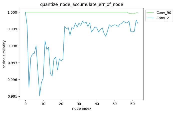
When average_mode = True:

average_mode_true_1

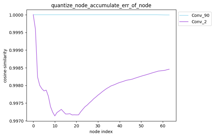
Note:

average_mode

average_mode defaults to False. For some models, the cumulative error curve may not clearly indicate which quantization strategy performs better under this setting. Therefore, setting average_mode to True can help by averaging the first n nodes’ cumulative errors as the cumulative error for the n-th node.

The specific calculation is as follows, for example:

When average_mode=False, accumulate_error=[1.0, 0.9, 0.9, 0.8].

When average_mode=True, accumulate_error=[1.0, 0.95, 0.933, 0.9].

Multiple Nodes Quantization

Configuration method: quantize_node=[['Conv_2'], ['Conv_2', 'Conv_90']], where quantize_node is a nested list.

API usage:

# Import debug module
import horizon_nn.quantizer.debugger as dbg

dbg.plot_acc_error(
        save_dir='./',
        calibrated_data='./calibration_data/',
        model_or_file='./calibrated_model.onnx',
        quantize_node=[['Conv_2'], ['Conv_2', 'Conv_90']],
        metric='cosine-similarity',
        average_mode=False)

Command-line usage:

  hmct-debugger plot-acc-error calibrated_model.onnx calibration_data -q [['Conv_2'],['Conv_2','Conv_90']]

Description: When quantize_node is a nested list, for each sublist in quantize_node, the nodes specified in that sublist are quantized while keeping all other nodes unquantized. After generating the corresponding models, the output of each node is compared with the corresponding node output in the floating-point model to compute the error, and the corresponding cumulative error curves are obtained.

partial_qmodel_0: Only quantize the Conv_2 node, leave others unquantized;
partial_qmodel_1: Only quantize the Conv_2 and Conv_90 nodes, leave others unquantized.

When average_mode=False:

new_average_mode_false_1

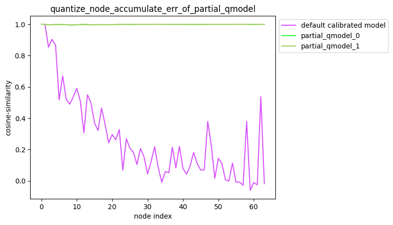
When average_mode=True:

new_average_mode_true_1

2. Cumulative Error Test After Dequantizing Specific Nodes in the Model

Single Node Dequantization

Configuration method: non_quantize_node=['Conv_2', 'Conv_90'], where non_quantize_node is a flat list.

API usage:

# Import debug module
import horizon_nn.quantizer.debugger as dbg

dbg.plot_acc_error(
        save_dir='./',
        calibrated_data='./calibration_data/',
        model_or_file='./calibrated_model.onnx',
        non_quantize_node=['Conv_2', 'Conv_90'],
        metric='cosine-similarity',
        average_mode=True)

Command-line usage:

  hmct-debugger plot-acc-error calibrated_model.onnx calibration_data -nq ['Conv_2','Conv_90'] -a True

Description: When non_quantize_node is a flat list, for each node in non_quantize_node, that node is dequantized (kept in float) while all other nodes remain quantized. After generating the corresponding models, the output of each node is compared with the corresponding node output in the floating-point model to compute the error, and the corresponding cumulative error curve is generated.

When average_mode = False:

average_mode_false_2

When average_mode = True:

average_mode_true_2

Multiple Nodes Dequantization

Configuration method: non_quantize_node=[['Conv_2'], ['Conv_2', 'Conv_90']], where non_quantize_node is a nested list.

API usage:

# Import debug module
import horizon_nn.quantizer.debugger as dbg

dbg.plot_acc_error(
        save_dir='./',
        calibrated_data='./calibration_data/',
        model_or_file='./calibrated_model.onnx',
        non_quantize_node=[['Conv_2'], ['Conv_2', 'Conv_90']],
        metric='cosine-similarity',
        average_mode=False)

Command-line usage:

  hmct-debugger plot-acc-error calibrated_model.onnx calibration_data -nq [['Conv_2'],['Conv_2','Conv_90']]

Description: When non_quantize_node is a nested list, for each sublist in non_quantize_node, the nodes in that sublist are kept unquantized while all other nodes are quantized. After generating the corresponding models, the output of each node is compared with the corresponding node output in the floating-point model to compute the error, and the corresponding cumulative error curves are obtained.

partial_qmodel_0: Do not quantize Conv_2, quantize all others;
partial_qmodel_1: Do not quantize Conv_2 and Conv_90, quantize all others.

When average_mode = False:

new_average_mode_false_2

When average_mode = True:

new_average_mode_true_2

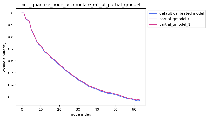
Testing Tips:

When testing partial quantization accuracy, you may want to compare multiple quantization strategies based on quantization sensitivity ranking. The following usage is recommended:

# Import debug module
import horizon_nn.quantizer.debugger as dbg

# First, use the sensitivity ranking function to get the sensitivity ranking of nodes in the model
node_message = dbg.get_sensitivity_of_nodes(
        model_or_file='./calibrated_model.onnx',
        metrics='cosine-similarity',
        calibrated_data='./calibration_data/',
        output_node=None,
        node_type='node',
        verbose=False,
        interested_nodes=None)
      
# node_message is a dictionary, with node names as keys
nodes = list(node_message.keys())

# Use `nodes` to specify non-quantized nodes for easy testing
dbg.plot_acc_error(
        save_dir='./',
        calibrated_data='./calibration_data/',
        model_or_file='./calibrated_model.onnx',
        non_quantize_node=[nodes[:1],nodes[:2]],
        metric='cosine-similarity',
        average_mode=True)

3. Separate Weight and Activation Quantization

Configuration method: quantize_node=['weight','activation'].

API usage:

import horizon_nn.quantizer.debugger as dbg

dbg.plot_acc_error(
        save_dir='./',
        calibrated_data='./calibration_data/',
        model_or_file='./calibrated_model.onnx',
        quantize_node=['weight','activation'],
        metric='cosine-similarity',
        average_mode=False)

Command-line usage:

  hmct-debugger plot_acc_error calibrated_model.onnx calibration_data -q ['weight','activation']

Description: quantize_node can directly specify 'weight' or 'activation'. Specifically:

quantize_node = ['weight']: Quantize only weights, not activations.
quantize_node = ['activation']: Quantize only activations, not weights.
quantize_node = ['weight', 'activation']: Quantize weights and activations separately.

weight_activation_quantized

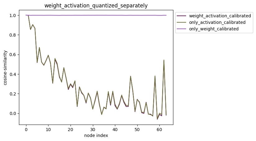
plot_distribution

Function: Select nodes and retrieve their outputs from both the floating-point model and the calibrated model to obtain output data distributions. Additionally, compute the difference between the two outputs to obtain the error distribution.

Command-line format:

hmct-debugger plot-distribution MODEL_OR_FILE CALIBRATION_DATA --other options

Use hmct-debugger plot-distribution -h/--help to view available parameters.

Parameter Table:

Parameter Name	Configuration Description	Value Range Description	Optional/Required
`save_dir or -s`	Function: Output directory. Description: Optional, specifies the path to save analysis results.	Range: Any valid path. Default: None.	Optional
`model_or_file`	Function: Specify calibrated model. Description: Required, specifies the calibrated model for analysis.	Range: Valid model path or ModelProto. Default: None.	Required
`calibrated_data`	Function: Specify calibration data. Description: Required, specifies the calibration data needed for analysis.	Range: Valid data path or CalibrationDataSet. Default: None.	Required
`nodes_list or -n`	Function: Specify nodes to analyze. Description: Required, specifies the nodes for analysis. For nodes in `nodes_list`: - Weight calibration nodes: Plot original and calibrated weight distributions. - Activation calibration nodes: Plot input data distribution of activation calibration nodes. - Ordinary nodes: Plot output distributions before and after quantization, and their error distribution. Note: `nodes_list` is of type List, allowing multiple nodes, and all three types can be specified simultaneously.	Range: All nodes in the calibrated model. Default: None.	Required

# Import debug module
import horizon_nn.quantizer.debugger as dbg

dbg.plot_distribution(
        save_dir: str, 
        model_or_file: ModelProto or str,
        calibrated_data: str or CalibrationDataSet,
        nodes_list: List[str] or str) 

Analysis Results Presentation:

API usage:

  # Import debug module
  import horizon_nn.quantizer.debugger as dbg

  dbg.plot_distribution(
          save_dir='./',
          model_or_file='./calibrated_model.onnx',
          calibrated_data='./calibration_data',
          nodes_list=['317_HzCalibration', # Activation node
                      '471_HzCalibration', # Weight node
                      'Conv_2']) # Ordinary node

Command-line usage:

hmct-debugger plot-distribution calibrated_model.onnx calibration_data -n ['317_HzCalibration','471_HzCalibration','Conv_2']

node_output:

node_output

weight:

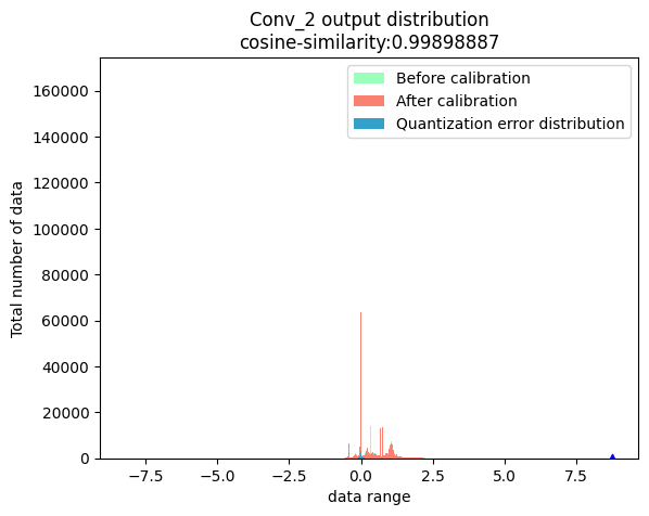
weight

activation:

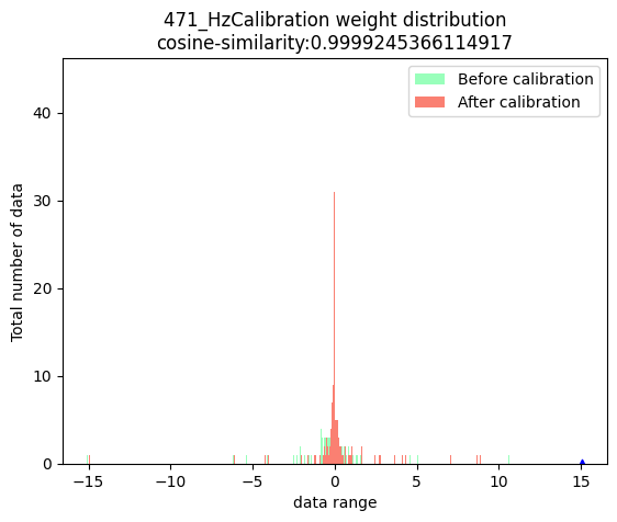
activation

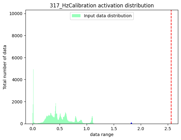
Note:

In the three figures above, the blue triangle represents the maximum absolute value of the data. The red dashed line represents the smallest calibration threshold.

get_channelwise_data_distribution

Function: Plot box plots showing channel-wise data distribution for specified calibration nodes.

Command-line format:

hmct-debugger get-channelwise-data-distribution MODEL_OR_FILE CALIBRATION_DATA --other options

Use hmct-debugger get-channelwise-data-distribution -h/--help to view parameters.

Parameter Table:

Parameter Name	Configuration Description	Value Range Description	Optional/Required
`save_dir or -s`	Function: Save path. Description: Optional, specifies the path to save results.	Range: Any valid path. Default: None.	Optional
`model_or_file`	Function: Specify calibrated model. Description: Required, specifies the model to analyze.	Range: Valid model path or ModelProto. Default: None.	Required
`calibrated_data`	Function: Specify calibration data. Description: Required, specifies the calibration data for analysis.	Range: Valid data path or CalibrationDataSet. Default: None.	Required
`nodes_list or -n`	Function: Specify calibration nodes. Description: Required, specifies the calibration nodes.	Range: All weight and activation calibration nodes in the model. Default: None.	Required
`axis or -a`	Function: Specify the dimension of channel. Description: The axis index where channel information resides. Default is None. For activation calibration nodes, assumes axis=1 (second dimension). For weight calibration nodes, reads the axis attribute from the node.	Range: Less than the input data dimension. Default: None.	Optional

# Import debug module
import horizon_nn.quantizer.debugger as dbg

dbg.get_channelwise_data_distribution(
        save_dir: str, 
        model_or_file: ModelProto or str,
        calibrated_data: str or CalibrationDataSet,
        nodes_list: List[str],
        axis: int = None)

Analysis Results Presentation:

Description: For each calibration node in nodes_list, extract channel-wise input data distribution using the axis parameter. By default, axis=None: for weight calibration nodes, channel dimension defaults to 0; for activation calibration nodes, defaults to 1.

Weight calibration node:

weight_calibration_node

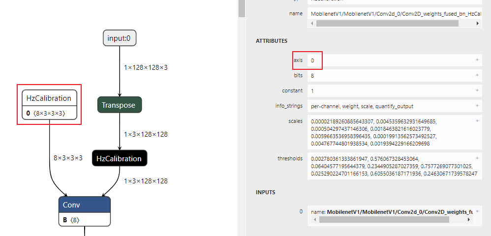
Activation calibration node:

activate_calibration_node

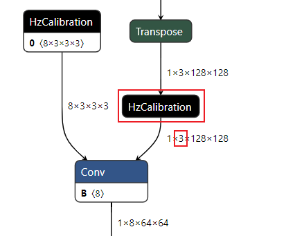
Output result as shown below:

box_plot

In the figure:

X-axis represents the number of channels in the node’s input data (e.g., 96 channels as shown in legend).
Y-axis represents the data distribution range per channel, where the red solid line indicates the median, and the blue dashed line indicates the mean.

sensitivity_analysis

Function: For quantization-sensitive nodes, analyze and test model accuracy when quantizing them individually or partially.

Command-line format:

hmct-debugger sensitivity-analysis MODEL_OR_FILE CALIBRATION_DATA --other options

Use hmct-debugger sensitivity-analysis -h/--help to view parameters.

Parameter Table:

Parameter Name	Configuration Description	Value Range Description	Optional/Required
`model_or_file`	Function: Specify calibrated model. Description: Required, specifies the model to analyze.	Range: Valid model path or ModelProto. Default: None.	Required
`calibrated_data`	Function: Specify calibration data. Description: Required, specifies data for analysis.	Range: Valid data path or CalibrationDataSet. Default: None.	Required
`pick_threshold or -p`	Function: Set sensitivity threshold for node selection. Description: Optional. Computes node quantization sensitivity and selects nodes with sensitivity below `pick_threshold` for analysis. Note: If `sensitive_nodes` is set, those nodes are tested directly without threshold-based selection.	Range: Any float. Default: 0.999.	Optional
`data_num or -d`	Function: Number of data samples for sensitivity computation. Description: Sets the number of data samples used to compute node sensitivity.	Range: >0 and ≤ total calibration data size. Default: 1.	Optional
`sensitive_nodes or -sn`	Function: Specify sensitive nodes for analysis. Description: Optional. Specifies nodes to analyze. If set, these nodes are tested directly.	Range: Any nodes in the calibrated model. Default: None.	Optional
`save_dir or -sd`	Function: Save path. Description: Optional, specifies where to save results.	Range: Any valid path. Default: None.	Optional

API usage:

# Import debug module
import horizon_nn.quantizer.debugger as dbg

dbg.sensitivity_analysis(model_or_file='calibrated_model.onnx',
                          calibrated_data='calibration_data',
                          pick_threshold=0.9999,
                          data_num=1,
                          sensitive_nodes=[])

Command-line usage:

hmct-debugger sensitivity-analysis calibrated_model.onnx calibration_data

Analysis Results Presentation:

activate_calibration_node

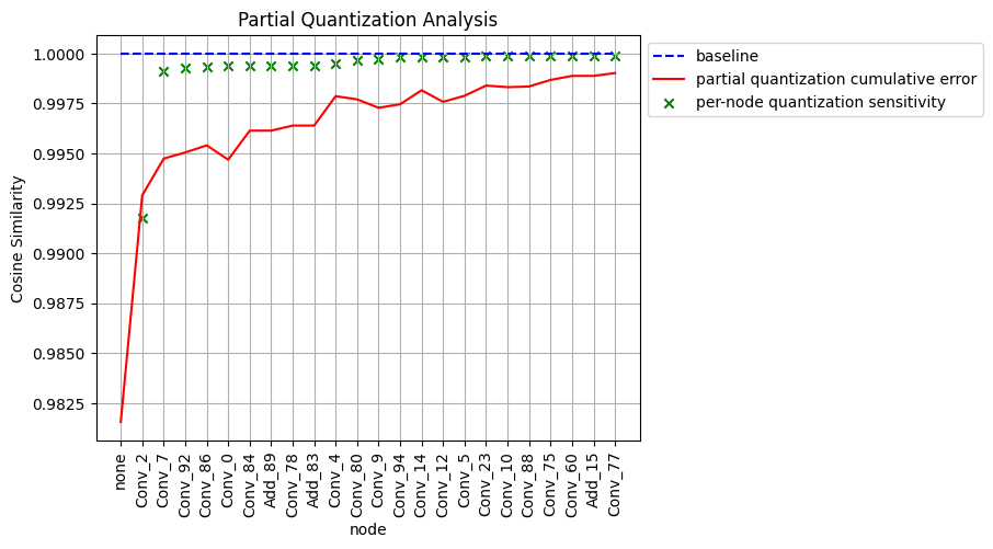
In the figure:

Blue dashed line: baseline, i.e., cosine similarity of the floating-point model output with itself, which is 1.
Green ‘x’: Quantize only the current node to get a partially quantized model; compute similarity between this model and the floating-point model.
Red solid line: Do not quantize the current node and all preceding nodes; compute similarity of the resulting partially quantized model with the floating-point model. For example, the similarity for Conv_92 is around 0.995, meaning that dequantizing Conv_2, Conv_7, and Conv_92 while keeping others quantized results in a model with ~0.995 cosine similarity. The first “none” on the x-axis in the red line refers to the fully calibrated model.

runall

Note:

The runall feature in the current version is only applicable to X5 products.

Function: Run all functionalities of the debug tool in one command.

Command-line format:

hmct-debugger runall MODEL_OR_FILE CALIBRATION_DATA --other options

Use hmct-debugger runall -h/--help to view parameters.

Parameter Table:

Parameter Name	Configuration Description	Value Range Description	Optional/Required
`model_or_file`	Function: Specify calibrated model. Description: Required, specifies the model to analyze.	Range: Valid model path or ModelProto. Default: None.	Required
`calibrated_data`	Function: Specify calibration data. Description: Required, specifies data for analysis.	Range: Valid data path or CalibrationDataSet. Default: None.	Required
`save_dir or -s`	Function: Save path. Description: Specifies where to save analysis results.	Range: Any valid path. Default: None.	Optional
`ns_metrics or -nm`	Function: Metric for node quantization sensitivity. Description: Specifies how to compute sensitivity. Can be a list to use multiple metrics, but sorting is based on the first metric. Higher rank means larger error introduced by quantizing the node.	Range: `'cosine-similarity'`, `'mse'`, `'mre'`, `'sqnr'`, `'chebyshev'`. Default: `'cosine-similarity'`.	Optional
`output_node or -o`	Function: Specify output node. Description: Allows specifying an intermediate node as output for sensitivity calculation. If None, uses the model's final output.	Range: Any node in the model with a calibration node. Default: None.	Optional
`node_type or -nt`	Function: Node type. Description: Type of nodes to compute sensitivity for: 'node' (ordinary), 'weight', 'activation'.	Range: `'node'`, `'weight'`, `'activation'`. Default: `'node'`.	Optional
`data_num or -dn`	Function: Number of data samples for sensitivity calculation. Description: Number of samples used. Default is None (use all calibration data). Minimum is 1.	Range: >0 and ≤ total calibration data size. Default: None.	Optional
`verbose or -v`	Function: Whether to print info to terminal. Description: If True, prints sensitivity info. If multiple metrics, sorted by the first.	Range: `True`, `False`. Default: `False`.	Optional
`interested_nodes or -i`	Function: Specify nodes of interest. Description: If set, only computes sensitivity for these nodes. Overrides `node_type`.	Range: Any nodes in the model. Default: None.	Optional
`dis_nodes_list or -dnl`	Function: Specify nodes to analyze. Description: Nodes for which to plot data distributions: - Weight calibration nodes: Plot original vs. calibrated weights. - Activation calibration nodes: Plot input data distribution. - Ordinary nodes: Plot output distribution before/after quantization and error. Note: `dis_nodes_list` is a list and can include multiple node types.	Range: All nodes in the model. Default: None.	Optional
`cw_nodes_list or -cn`	Function: Specify calibration nodes. Description: Nodes for which to plot channel-wise distributions.	Range: All weight and activation calibration nodes. Default: None.	Optional
`axis or -a`	Function: Specify channel dimension. Description: Axis index of channel. Default is None: for activation nodes, assumes axis=1; for weight nodes, reads from node attribute.	Range: Less than input data dimension. Default: None.	Optional
`quantize_node or -qn`	Function: Quantize only specified nodes and observe cumulative error. Description: Optional. Specifies nodes to quantize, others remain unquantized. Whether single or partial quantization depends on whether the input is a nested list. Examples: - `quantize_node=['Conv_2','Conv_9']`: Quantize Conv_2 and Conv_9 individually. - `quantize_node=[['Conv_2'],['Conv_9','Conv_2']]`: Test quantizing Conv_2 alone and both Conv_2 & Conv_9. Special values: 'weight', 'activation': - `['weight']`: Quantize only weights. - `['activation']`: Quantize only activations. - `['weight','activation']`: Quantize both separately. Note: `quantize_node` and `non_quantize_node` cannot both be None; at least one must be specified.	Range: All nodes in the model. Default: None.	Optional
`non_quantize_node or -nqn`	Function: Specify nodes to keep unquantized for cumulative error test. Description: Optional. Nodes to keep in float, others fully quantized. Determines single or multiple dequantization based on whether input is nested. Examples: - `non_quantize_node=['Conv_2','Conv_9']`: Dequantize Conv_2 and Conv_9 individually. - `non_quantize_node=[['Conv_2'],['Conv_9','Conv_2']]`: Dequantize Conv_2 alone and both Conv_2 & Conv_9. Note: One of `quantize_node` or `non_quantize_node` must be specified.	Range: All nodes in the model. Default: None.	Optional
`ae_metric or -am`	Function: Cumulative error metric. Description: Sets the method for calculating model error.	Range: `'cosine-similarity'`, `'mse'`, `'mre'`, `'sqnr'`, `'chebyshev'` Default: `'cosine-similarity'`.	Optional
`average_mode or -avm`	Function: Specifies the output mode for the cumulative error curve. Description: Default is False. If set to True, the average of the cumulative error is used as the result.	Range: `True`, `False`. Default: `False`.	Optional
`pick_threshold or -pt`	Function: Sets the sensitivity threshold for selecting nodes. Description: Optional. This feature calculates the quantization sensitivity of regular nodes and selects nodes with sensitivity lower than pick_threshold as sensitive nodes for analysis and testing. Note: When sensitive_nodes is set, the nodes specified in sensitive_nodes are tested directly, without recalculating node sensitivity or selecting sensitive nodes based on pick_threshold.	Range: None. Default: 0.999.	Optional
`sensitive_nodes or -sn`	Function: Specifies the sensitive nodes to be analyzed. Description: Optional. Specifies the sensitive nodes to be analyzed. Note: When this parameter is set, the nodes specified in this parameter are tested directly, without recalculating node sensitivity or selecting sensitive nodes based on pick_threshold.	Range: All nodes in the calibrated model. Default: None.	Optional

API Usage:

# Import debug module
import horizon_nn.quantizer.debugger as dbg

dbg.runall(model_or_file='calibrated_model.onnx',
            calibrated_data='calibration_data')

Command-line Usage:

hmct-debugger runall calibrated_model.onnx calibration_data

runall Workflow:

runall

When all parameters remain at their defaults, the tool performs the following steps sequentially:

Step 1 and Step 2: Obtain quantization sensitivity for weight calibration nodes and activation calibration nodes, respectively.
Step 3: Based on results from Step 1 and Step 2, plot data distributions for the top 5 weight calibration nodes and top 5 activation calibration nodes.
Step 4: For the nodes obtained in Step 3, plot box plots showing inter-channel data distributions.
Step 5: Plot cumulative error curves for quantizing weights only and activations only.
Step 6: Perform partial quantization and per-node accuracy analysis on sensitive nodes. Since the example in the figure does not specify sensitive_nodes, the debug tool must compute quantization sensitivity of regular nodes and select nodes with sensitivity below the specified pick_threshold for testing and analysis.

When node_type='node' is specified, the tool retrieves the top 5 nodes, finds the corresponding calibration nodes for each, and obtains their data distribution and box plots.

6.3.2.7. Improving Model Accuracy Using QAT (Quantization-Aware Training)

If, after the above analysis, no configuration issues are found but accuracy still does not meet requirements, the limitation may lie in PTQ (Post-Training Quantization). In this case, we can switch to QAT for model quantization.

Horizon Plugin PyTorch follows PyTorch’s official quantization API and design principles, adopting the Quantization Aware Training (QAT) approach. We recommend reading the QAT section in the PyTorch official documentation.

For a more detailed introduction to Horizon Plugin PyTorch, please refer to the Advanced Guide - QAT Quantization-Aware Training section.

Based on previous optimization experience, the above strategies can handle various practical issues.

If your issue remains unresolved after trying the above steps, please follow the Accuracy Optimization Checklist document to fill in specific model configuration details, ensure all troubleshooting steps are completed, identify the exact step in model conversion where anomalies occur, and then submit the completed accuracy optimization checklist, the original floating-point model file, model quantization configuration files, and other relevant information to the technical support team or post your question on the Official Technical Community. We will provide support within 24 hours.

6.3.2.8. Other Tool Usage Instructions

This section introduces the usage of other debug tools beyond the model conversion tools. These tools assist developers in model modification, model analysis, data preprocessing, and other operations. The tool list is as follows:

hb_mapper infer
hb_perf
hb_pack
hb_model_info
hb_model_modifier
hb_verifier
hb_eval_preprocess
HB_ONNXRuntime Inference Library

`hb_mapper infer` Tool

Note:

Due to onnxruntime limitations, hb_mapper infer does not support dynamic shape inference, so the input model must have explicit shape information.
This tool does not support infer on models with shape information marked as “?”.
This tool only supports non-featuremap models with four-dimensional inputs and outputs of four dimensions or fewer.

This command performs inference using both floating-point and quantized models and saves the inference results to the directory specified by --output-dir.

To verify and analyze whether model compilation is correct, set layer_out_dump in the configuration file to True, which will output inference results of conv and output nodes. Then, use vector comparison tools to analyze the correctness of model compilation.

Usage

hb_mapper infer usage:

  hb_mapper infer --config ${config_file} \
                  --model-file ${quantized_model_file}  \
                  --model-type ${caffe/onnx} \
                  --image-file ${input_node} ${image_file} \
                  --input-layout ${input_layout} \
                  --output-dir ${quantized_output_dir}

When using the hb_mapper infer command, use the same configuration file as in the hb_mapper makertbin command to ensure consistent input data processing settings. In short, the images or data used for calibration in hb_mapper makertbin should be in the same format when used in hb_mapper infer.

Note: The choice of input data in the hb_mapper infer command is related to the following input data configuration in the configuration file:

If preprocess_on: True, the tool can accept JPEG images, automatically perform resizing and other preprocessing, and convert them into the input_type_rt format.
If preprocess_on: False, it can only accept preprocessed binary image files. Therefore, preprocessing must be done manually, and images must be converted into corresponding binary files. (Refer to script 02_preprocess.sh).

Command-line Arguments

-h, –help Show help message and exit.

-c, –config Configuration file used during model compilation.

–model-file Model file for inference; can be a floating-point or quantized ONNX model.

–model-type Specify the type of the original floating-point model for inference; can be caffe or onnx.

–image-file Input node name and its corresponding image file for inference.

–input-layout Layout of the model input (optional).

–output-dir Path to save inference results. For quantized models, results are dequantized floating-point data.

Output files are saved in the output_dir directory, named according to the rule: ${layername}_float.bin.

`hb_perf` Tool

hb_perf is a tool for analyzing the performance of X5 algorithm chain quantized hybrid models.

Usage

hb_perf [OPTIONS] BIN_FILE

Command-line Arguments

hb_perf command-line arguments:

–version
Show version and exit.

-m
Followed by model name. When BIN_FILE is a packed model, only outputs compilation information for the specified model.

–help
Show help information.

Output Description

Model information is output to the hb_perf_result folder in the current directory. A folder named after the model will be created, and model information will be displayed in an HTML file named after the model. The directory structure is shown in the example below:

  hb_perf_result/
  └── mobilenetv1
      ├── mobilenetv1
      ├── mobilenetv1.html
      ├── mobilenetv1.png
      ├── MOBILENET_subgraph_0.html
      ├── MOBILENET_subgraph_0.json
      └── temp.hbm

If the model was not compiled in debug mode (compiler_parameters.debug:True), hb_perf will display the following warning. This warning only indicates that subgraph information does not include per-layer details and does not affect the generation of overall model information.

2021-01-12 10:41:40,000 WARNING bpu model don't have per-layer perf info.
2021-01-12 10:41:40,000 WARNING if you need per-layer perf info please enable[compiler_parameters.debug:True] when use makertbin.

`hb_pack` Tool

hb_pack is a tool for packaging multiple hybrid model (*.bin) files into a single model file.

Usage

hb_pack [OPTIONS] BIN_FILE1 BIN_FILE2 BIN_FILE3 -o comb.bin

Command-line Arguments

hb_pack command-line arguments:

–version
Show version and exit.

-o, –output_name
Output name for the packed model.

–help
Show help information.

Output Description

The packed model is output to the current directory, named as specified by output_name. Compilation and performance information of all submodels in the packed model can be obtained using hb_model_info and hb_perf.

Note: Note that hb_pack does not support repacking already packed models; otherwise, the following message will appear:

ERROR exception in command: pack
ERROR model: xxx.bin is a packed model, it can not be packed again!

`hb_model_info` Tool

hb_model_info is a tool for parsing dependency and parameter information of hybrid models (*.bin) during compilation.

Usage

  hb_model_info ${model_file}

Command-line Arguments

hb_model_info command-line arguments:

–version
Show version and exit.

-m
Followed by model name. When BIN_FILE is a packed model, only outputs compilation information for the specified model.

–help
Show help information.

Output Description

Output includes some input information during model compilation, as shown below:

Note: Version information in the code block below varies with release packages; this is just an example.

Start hb_model_info....
hb_model_info version 1.3.35
******** efficient_det_512x512_nv12 info *********
############# model deps info #############
hb_mapper version   : 1.3.35
hbdk version        : 3.23.3
hbdk runtime version: 3.13.7
horizon_nn version  : 0.10.10
############# model_parameters info #############
onnx_model          : /release/01_common/model_zoo/mapper/detection/efficient_det/efficientdet_nhwc.onnx
BPU march           : bernoulli2
layer_out_dump      : False
working dir         : /release/04_detection/05_efficient_det/mapper/model_output
output_model_file_prefix: efficient_det_512x512_nv12
############# input_parameters info #############
------
---------input info : data ---------
input_name          : data
input_type_rt       : nv12
input_space&range   : regular
input_layout_rt     : None
input_type_train    : rgb
input_layout_train  : NCHW
norm_type           : data_mean_and_scale
input_shape         : 1x3x512x512
mean_value          : 123.68,116.779,103.939,
scale_value         : 0.017,
cal_data_dir        : /release/04_detection/05_efficient_det/mapper/calibration_data_rgb_f32
---------input info : data end -------
------
############# calibration_parameters info #############
preprocess_on       : False
calibration_type    : max
############# compiler_parameters info #############
hbdk_pass_through_params: --fast --O3
input-source        : {'data': 'pyramid', '_default_value': 'ddr'}
--------- input/output types -
model input types   : [<InputDataType.NV12: 7>]
model output types  : [<InputDataType.F32: 5>, <InputDataType.F32: 5>, <InputDataType.F32: 5>, <InputDataTye.F32: 5>, <InputDataType.F32: 5>, <InputDataType.F32: 5>, <InputDataType.F32: 5>, <InputDataType.F32: 5>, <InputDataType.F32: 5>, <InpuDataType.F32: 5>]

Note:

When deleted nodes exist in the model, their names are printed at the end of the model information output, and a deleted_nodes_info.txt file is generated, with each line recording the initial information of a corresponding deleted node. Example output of deleted node names:

--------- deleted nodes -
deleted nodes: spconvretinanethead0_conv91_fwd_chw_HzDequantize
deleted nodes: spconvretinanethead0_conv95_fwd_chw_HzDequantize
deleted nodes: spconvretinanethead0_conv99_fwd_chw_HzDequantize
deleted nodes: spconvretinanethead0_conv103_fwd_chw_HzDequantize
deleted nodes: spconvretinanethead0_conv107_fwd_chw_HzDequantize
deleted nodes: spconvretinanethead0_conv93_fwd_chw_HzDequantize
deleted nodes: spconvretinanethead0_conv97_fwd_chw_HzDequantize
deleted nodes: spconvretinanethead0_conv101_fwd_chw_HzDequantize
deleted nodes: spconvretinanethead0_conv105_fwd_chw_HzDequantize
deleted nodes: spconvretinanethead0_conv109_fwd_chw_HzDequantize

`hb_model_modifier` Tool

hb_model_modifier is a tool for removing Transpose and Quantize nodes at the input side and Transpose, Dequantize, Cast, Reshape, Softmax nodes at the output side of a *.bin model. Information about removed nodes is stored within the BIN model and can be viewed via hb_model_info.

Note:

hb_model_modifier can only remove nodes immediately adjacent to model inputs or outputs. If the node to be removed is followed by other nodes, deletion is not allowed.
Model node names should not contain special characters such as “;” or “,”, which may affect tool usage.
The tool does not support processing packed models; otherwise, it will prompt: ERROR pack model is not supported.
Nodes to be removed are deleted sequentially, and the model structure is dynamically updated; before deletion, the tool checks whether the node is located at the model’s input or output. Therefore, the deletion order matters.

Because removing specific nodes may affect model input, the tool is only suitable for models with a single path after input. Cases where one input connects to multiple nodes (as shown in the figure below) are currently unsupported.

hb_model_modifier

Usage

View removable nodes:
```
hb_model_modifier model.bin
```
Remove a single specified node (e.g., node1):
```
hb_model_modifier model.bin -r node1
```

Remove multiple specified nodes (e.g., node1, node2, node3):

hb_model_modifier model.bin -r node1 -r node2 -r node3

Remove all nodes of a certain type (e.g., Dequantize):
```
hb_model_modifier model.bin --all Dequantize
```

Remove multiple types of nodes (e.g., Reshape, Cast, Dequantize):

hb_model_modifier model.bin -a Reshape -a Cast -a Dequantize

Combined usage:

hb_model_modifier model.bin -a Reshape -a Cast -a Dequantize -r node1 -r node2 -r node3

Command-line Arguments

hb_model_modifier command-line arguments:

–model_file
Runtime model file name.

-r
Followed by the name of the node to be removed. For multiple nodes, specify this option multiple times.

-o
Followed by the output name of the modified model (only effective when -r is used).

-a –all
Followed by node type. Supports batch removal of all nodes of the specified type. For multiple types, specify this option multiple times.

Output Description

If no arguments are provided, the tool prints all candidate removable nodes (i.e., all Transpose, Quantize, Dequantize, Cast, Reshape, Softmax nodes located at input/output positions).

The Quantize node converts model input data from float type to int8 type using the following formula:

  qx = clamp(round(x / scale) + zero_point, -128, 127)

round(x) rounds floating-point numbers to the nearest integer, clamp(x) clamps values to integers between -128 and 127. zero_point is the asymmetric quantization zero-point offset; for symmetric quantization, zero_point = 0.

C++ reference implementation:

  int64_t quantized_value =
      static_cast<int64_t>(std::round(value / static_cast<double>(scale)));
  quantized_value = std::min(std::max(quantized_value, min_int_value), max_int_value);

The Dequantize node converts model output data from int8 or int32 type back to float or double type using the formula:

  deqx = (x - zero_point) * scale

C++ reference implementation:

  static_cast<float>(value) * scale

Note:

Currently, the tool supports removing:

Quantize or Transpose nodes at input positions;
Transpose, Dequantize, Cast, Reshape, Softmax nodes at output positions.

Tool output example:

hb_model_modifier resnet50_64x56x56_featuremap.bin
2022-04-21 18:22:30,207 INFO Nodes that can be deleted: ['data_res2a_branch1_HzQuantize_TransposeInput0', 'fc1000_reshape_0']

After specifying the -r option, the tool prints the node type, information stored in the bin file, and confirms the node has been removed:

hb_model_modifier resnet50_64x56x56_featuremap.bin -r data_res2a_branch1_HzQuantize_TransposeInput0
Node 'data_res2a_branch1_HzQuantize_TransposeInput0' found, its OP type is 'Transpose'
Node 'data_res2a_branch1_HzQuantize_TransposeInput0' is removed
modified model saved as resnet50_64x56x56_featuremap_modified.bin

Then, use hb_model_info to view deleted node information. The end of the output will list the names of deleted nodes, and a deleted_nodes_info.txt file will be generated, with each line recording initial information of the corresponding deleted node. Example:

hb_model_info resnet50_64x56x56_featuremap_modified.bin
Start hb_model_info....
hb_model_info version 1.7.0
********* resnet50_64x56x56_featuremap info *********
...
--------- deleted nodes -
deleted nodes: data_res2a_branch1_HzQuantize_TransposeInput0

`hb_verifier` Tool

hb_verifier is a tool for verifying results of specified fixed-point models and runtime models.

If you specify images before using the tool, hb_verifier will perform inference on the fixed-point model, and on the runtime model both on-device and on the X86 simulator, then perform pairwise comparisons of results and provide a pass/fail conclusion (this process is optional; you can choose which comparisons to perform based on needs).

The tool uses the specified images to perform inference on the fixed-point model, runtime model on-device, and runtime model on the X86 simulator. Runtime model inference on-device is performed if the given IP is reachable and hrt_tools is installed on the board (if not, install using the install.sh script under package/board in the toolchain SDK package). Runtime model inference on the X86 host is performed if hrt_tools is installed on the host (if not, install using the install.sh script under package/host in the toolchain SDK package). The tool then performs pairwise comparisons of all three results and provides a pass/fail conclusion. If no image is specified, the tool uses default images for inference (for featuremap models, random tensor data is generated).

Note:

For instructions on obtaining the package, refer to Delivery Description.
hb_verifier does not support comparing bin models (with node changes other than Dequantize nodes) with quanti.onnx.

If before using this tool, you used hb_model_modifier to remove the last node before output in the bin model and that node is not a Dequantize node, or if the YAML file contains the remove_node_type parameter that removes the last node before output and that node is not a Dequantize node, then hb_verifier will no longer support comparing quanti.onnx with the modified bin model.

To resolve this issue, avoid removing the last node before output in the bin model if it is not a Dequantize node.
Since hb_verifier interacts with the board via SSH, if you use this tool inside a Docker container, do not use the docker attach command to connect to the container, as it will cause SSH authentication with the board to fail.

Usage

hb_verifier -m   ${quanti_model},${bin_model} \
            -b   ${board_ip} \
            -s   True / False \  
            -i   ${input_img} \ 
            -c   ${digits}  \
            -r   True / False
            -u   Board username
            -p   Board password

Command-line Arguments

hb_verifier command-line arguments:

–version Show version and exit.

-h, –help Show help information.

-m, –model Name of the fixed-point model and bin model, separated by “,” for multiple models.

-b, –board-ip ARM board IP address for on-device testing.

-s, –run-sim Set whether to use libdnn in X86 environment for bin model inference, default is False.

- When set to ``True``, the tool will use libdnn in the X86 environment for bin model inference.    - When this parameter is set to ``False``, the tool will not use the libdnn from the x86 environment for bin model inference.

-i, –input-img Specify the image used for inference testing.

If not specified, randomly generated tensor data will be used.

If the specified image is in binary format, the file must have the ``.bin`` extension.

For models with multiple inputs, there are two ways to pass images; multiple images should be separated by commas:

    - input_name1:image1,input_name2:image2, ...

    - image1,image2...

Note: In multi-batch model scenarios, the hb_verifier tool does not support input configured as binary data. It is recommended to either specify a single-batch image or leave the input unspecified to use random data for consistency verification.

-c, –compare_digits Set the numerical precision (i.e., number of decimal places) for comparing inference results. If not specified, the tool defaults to comparing up to five decimal places.

-r, –dump-all-nodes-results Determine whether to save the output results of each operator in the model and compare results with identical operator output names. Default is False.

- When this parameter is set to ``True``, the tool will obtain outputs from all nodes in the model and perform comparisons based on matching node output names.

- When this parameter is set to ``False``, the tool will only retrieve and compare the final output results of the model.

Note: Please note that, for performance considerations, the dump functionality is currently not supported when using the tool in an X86 environment.

-u, –username Specify the username for the development board. Default is root.

-p, –password Enter the password for the development board if it is password-protected.

Note: If your development board does not have a password set, please do not provide this option.

Example Usage Scenarios

Perform inference on quanti.onnx model and bin model on the development board, perform inference on the bin model in the X86 environment, and compare the inference results from all three:
```
hb_verifier -m quanti.onnx,model.bin -b *.*.*.* -s True (-i optional)
```
Perform inference on quanti.onnx model and bin model on the development board, and compare the inference results from both:
```
hb_verifier -m quanti.onnx,model.bin -b *.*.*.* (-i optional)
```
Perform inference on quanti.onnx model and bin model on the development board, while saving outputs of all operators in both models and comparing results with identical operator output names:
```
hb_verifier -m quanti.onnx,model.bin -b *.*.*.* -r True (-i optional)
```
Perform inference on quanti.onnx model and bin model in the X86 environment, and compare the inference results from both:
```
hb_verifier -m quanti.onnx,model.bin -s True (-i optional)
```
- Output Description
The comparison results will ultimately be displayed in the terminal. The tool compares the execution results of multiple models under different scenarios. If no issues are found, the output should appear as follows:
```
  Comparison results of original output is model_infer_output_0
  raw output 0 and raw output 0 result Strict check PASSED
  Quanti.onnx and Arm result Strict check PASSED
```

When there is a precision mismatch between fixed-point and runtime models, detailed information about the mismatch will be displayed, as shown in the log below:

  INFO ================== Sim infer log end ==========================
  INFO ***************************************************************
  INFO compare source: Quanti.onnx VS Arm
  INFO compare model name: clr_320x800_bgr_quantized_model VS clr_320x800_bgr
  Compare progress: 100%|###########################| 1/1 [00:00<00:00, 55.47it/s]
  INFO =============== Original output comparison results =================
  INFO Comparison results of original output is model_infer_output_0_output
  INFO mismatch result num: 1000
  INFO total result num: 1000
  INFO mismatch rate: 1.0
  INFO relative mismatch ratio: 0.9997149805034536
  INFO max abs error: 8.36695
  WARNING raw output output and raw output output result Strict check FAILED
  WARNING Quanti.onnx and Arm result Strict check FAILED
  INFO ***************************************************************
  INFO ***************************************************************
  INFO compare source: Quanti.onnx VS Sim
  INFO compare model name: clr_320x800_bgr_quantized_model VS clr_320x800_bgr
  Compare progress: 100%|##########################| 1/1 [00:00<00:00, 135.53it/s]
  INFO =============== Original output comparison results =================
  INFO Comparison results of original output is model_infer_output_0_output
  INFO mismatch result num: 1000
  INFO total result num: 1000
  INFO mismatch rate: 1.0
  INFO relative mismatch ratio: 0.9997149805034536
  INFO max abs error: 8.36695
  WARNING raw output output and raw output output result Strict check FAILED
  WARNING Quanti.onnx and Sim result Strict check FAILED
  INFO ***************************************************************
  INFO ***************************************************************
  INFO compare source: Arm VS Sim
  INFO compare model name: clr_320x800_bgr VS clr_320x800_bgr
  Compare progress: 100%|##########################| 1/1 [00:00<00:00, 150.69it/s]
  INFO Arm and Sim result Strict check PASSED
  INFO ***************************************************************

Where:

mismatch result num indicates the number of mismatched results between the two models, including three types of mismatches:
- mismatch.line_miss num: the number of cases where the count of output results differs.
- mismatch.line_diff num: the number of cases where the output results differ significantly.
- mismatch.line_nan num: the number of cases where outputs are NaN.
total result num is the total number of output data points.
mismatch rate is the ratio of mismatched data points to the total number of output data points.
relative mismatch ratio is the relative error ratio, showing the maximum value among all error ratios.
max abs error is the maximum absolute error.

`hb_eval_preprocess` Tool

Used for preprocessing image data in the x86 environment when evaluating model accuracy.
Preprocessing refers to specific operations performed on image data before feeding it into the model, such as resizing, cropping, and padding.

Usage
```
  hb_eval_preprocess [OPTIONS]
```

Command-line Arguments

Command-line arguments for hb_eval_preprocess:

  --version<br/>
    Show version and exit.

  -m, --model_name<br/>
    Set the model name. Supported models can be viewed via ``hb_eval_preprocess --help``.

  -i, --image_dir<br/>
    Input image directory.

  -o, --output_dir<br/>
    Output directory.

  -v, --val_txt<br/>
    Specify the file containing image names required for evaluation. The preprocessed images will correspond to the image names listed in this file.

  -h, --help<br/>
    Show help information.

Output Description

The hb_eval_preprocess command will generate image binary files in the path specified by --output_dir.

Tip: For more examples of using the hb_eval_preprocess tool in model accuracy evaluation on embedded devices, refer to the Data Preprocessing section in the Embedded Application Development guide titled “General Model Evaluation Instructions”.

`HB_ONNXRuntime` Inference Library

HB_ONNXRuntime is a x86-side ONNX model inference library developed by Horizon Robotics, built upon the open-source ONNXRuntime. It supports not only original ONNX models directly exported from training frameworks such as PyTorch, TensorFlow, PaddlePaddle, and MXNet, but also intermediate ONNX models generated during the PTQ (Post-Training Quantization) conversion process using Horizon’s toolchain. The usage flow is shown in the diagram below:

hb_onnxruntime

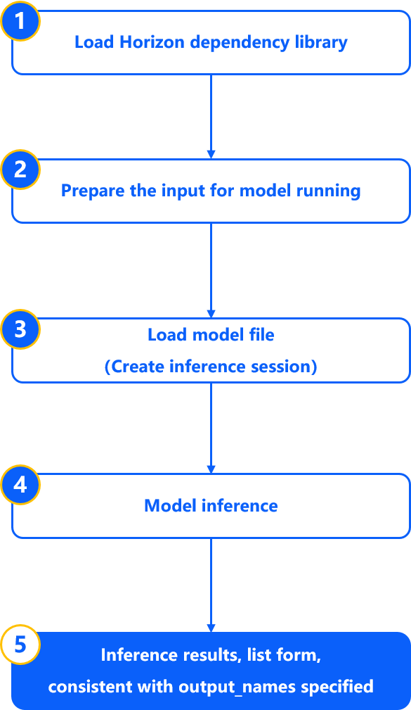
Note:

Please note that computing platforms based on the X5 BPU architecture use int8 computation precision (a common standard across industry platforms). During PTQ conversion using the X5 algorithm toolchain, although the final generated bin model handles input_type_rt to input_type_train color space conversion in hardware, the preprocessing nodes inserted at the front end of intermediate ONNX models (excluding featuremap inputs and when norm_type is not configured as no_preprocess) do not include hardware-level conversion logic. Therefore, the actual input to the ONNX model is an intermediate type (for non-featuremap inputs, a -128 adjustment is required, i.e., converting from uint8 to int8). HB_ONNXRuntime internally handles such data conversions, but only for non-lossy conversion scenarios as follows:

Model input type is int8: supports input as int8 or uint8.
Model input type is uint8: supports input as int8 or uint8.
Model input type is float32: supports input as int8, uint8, or float32.

For mixed-type inputs or other cases involving lossy conversions, users must manually handle the corresponding data transformations before performing inference.

Usage

The basic workflow for loading and running ONNX models using HB_ONNXRuntime is shown below. This example code applies to inference for all ONNX models; simply prepare data according to the model’s input type and layout requirements:

import numpy as np
# Load Horizon Robotics dependency
from horizon_tc_ui import HB_ONNXRuntime
# Prepare input for model execution
input_data = np.load("input.npy")
# Load the model file
sess = HB_ONNXRuntime(model_file = "model.onnx")
# Retrieve input and output node information
input_names = sess.input_names
output_names = sess.output_names
# Prepare input data; assuming this model has only one input
input_info = {input_names[0]: input_data}
# Perform inference; the return value is a list corresponding to output_names in order
output = sess.run(output_names, input_info)

Parameter Description

output_names:

Configures the output names and supports being set to None or custom-defined.

If set to None, the tool internally reads the model’s output node information and returns inference results in parsing order.

If custom-defined, you may specify all or a subset of output names, and reorder them. The inference results will then be returned according to your specified names and order.

input_info:

Prepare input data according to the model’s input type and layout. The configuration must be in dictionary format, with input names and corresponding data as key-value pairs. Example: {”input_name”: data}.

6.3.2. PTQ Principle and Step-by-Step Guide

6.3.2.1. Introduction

6.3.2.2. Model Preparation

6.3.2.3. Model Verification

Using the hb_mapper checker Tool to Verify Models

Handling Verification Exceptions

Interpreting Verification Results

Optimization Guidance from Verification Results

6.3.2.4. Model Conversion

Preparing Calibration Data

Using the hb_mapper makertbin Tool for Model Conversion

Model Conversion YAML Configuration Parameters

Model parameter group

Enter information parameter group

Calibration parameter group

Compile parameter group

Custom operator parameter group

X5 int16 configuration instructions

Instructions for preprocessing HzPreprocess operator

[Reference] Supported calibration methods

Interpretation internal process

Interpretation of conversion results

Interpretation of Conversion Outputs

6.3.2.5. Model Performance Analysis

Performance Evaluation on Development Machine

Performance Measurement on Development Board

Model Performance Optimization

Check YAML Parameters Affecting Model Performance

Handling CPU Operators

High-Performance Model Design Recommendations

6.3.2.6. Model Accuracy Analysis

Accuracy Analysis

Accuracy Optimization

Significant Accuracy Loss (Over 4%)

Minor Accuracy Loss Optimization (1.5%~3%)

Accuracy Debug Tool

Usage Instructions

Function Description

get_sensitivity_of_nodes

plot_acc_error

plot_distribution

get_channelwise_data_distribution

sensitivity_analysis

6.3.2.7. Improving Model Accuracy Using QAT (Quantization-Aware Training)

6.3.2.8. Other Tool Usage Instructions

hb_mapper infer Tool

hb_perf Tool

hb_pack Tool

hb_model_info Tool

hb_model_modifier Tool

hb_verifier Tool

hb_eval_preprocess Tool

HB_ONNXRuntime Inference Library

Using the `hb_mapper checker` Tool to Verify Models

`hb_mapper infer` Tool

`hb_perf` Tool

`hb_pack` Tool

`hb_model_info` Tool

`hb_model_modifier` Tool

`hb_verifier` Tool

`hb_eval_preprocess` Tool

`HB_ONNXRuntime` Inference Library