6.4.4. In-Depth Exploration
6.4.4.1. FX Quantization Principle Introduction
Before reading this document, it is recommended to first read torch.fx — PyTorch documentation to gain a basic understanding of PyTorch’s FX mechanism.
FX uses symbolic execution to build computational graphs at the level of nn.Module or functions, enabling automated operator fusion and other graph-based optimizations.
Quantization Workflow
Fuse (Optional)
FX is aware of the computation graph, so it enables automatic operator fusion. Users no longer need to manually specify which operators to fuse—simply call the API.
fused_model = horizon.quantization.fuse_fx(model)
Note that
fuse_fxdoes not have aninplaceparameter, because internally it performs symbolic tracing to generate aGraphModule, which cannot modify the model in-place.fused_modelandmodelwill share almost all attributes (including submodules, operators, etc.), so do not modifymodelafter fusion, as it may affectfused_model.Users do not need to explicitly call
fuse_fx, as the subsequentprepare_qat_fxAPI internally integrates the fusion process.
Prepare
Before calling prepare_qat_fx, users must set the global march according to the target hardware platform. Internally, the API first performs fusion (even if the model has already been fused), then replaces eligible operators in the model with implementations from horizon.nn.qat.
Users can choose an appropriate qconfig based on their needs (Calibration or QAT; note that these two types of qconfig cannot be mixed).
Similar to
fuse_fx, this API does not support theinplaceparameter. Afterprepare_qat_fx, do not modify the input model.
# Set march: **X3** to BERNOULLI2, **X5** to BAYES_E.
horizon.march.set_march(horizon.march.March.BAYES_E)
qat_model = horizon.quantization.prepare_qat_fx(
    model,
    {
        "": horizon.qconfig.default_calib_8bit_fake_quant_qconfig,
        "module_name": {
            "<module_name>": custom_qconfig,
        },
    },)
Convert
Similar to
fuse_fx, this API does not support theinplaceparameter. Afterconvert_fx, do not modify the input model.
quantized_model = horizon.quantization.convert_fx(qat_model)
Eager Mode Compatibility
In most cases, FX quantization APIs can directly replace eager mode quantization APIs (prepare_qat → prepare_qat_fx, convert → convert_fx), but they cannot be mixed with eager mode APIs. Some models require code structure modifications under the following circumstances:
Unsupported operations by FX: Symbolic tracing in PyTorch supports only a limited set of operations. For example, non-static variables cannot be used as conditional statements, and packages outside of PyTorch (e.g., NumPy) are not supported by default. Additionally, branches not executed during tracing are discarded.
Operations not intended for FX processing: If torch ops are used in model preprocessing or postprocessing, FX will treat them as part of the model during tracing, potentially causing unexpected behavior (e.g., replacing certain torch function calls with
FloatFunctional).
Both scenarios can be avoided using the “wrap” method. The RetinaNet example below illustrates this.
from horizon_plugin_pytorch.utils.fx_helper import wrap as fx_wrap

class RetinaNet(nn.Module):
    def __init__(
        self,
        backbone: nn.Module,
        neck: Optional[nn.Module] = None,
        head: Optional[nn.Module] = None,
        anchors: Optional[nn.Module] = None,
        targets: Optional[nn.Module] = None,
        post_process: Optional[nn.Module] = None,
        loss_cls: Optional[nn.Module] = None,
        loss_reg: Optional[nn.Module] = None,
    ):
        super(RetinaNet, self).__init__()

        self.backbone = backbone
        self.neck = neck
        self.head = head
        self.anchors = anchors
        self.targets = targets
        self.post_process = post_process
        self.loss_cls = loss_cls
        self.loss_reg = loss_reg

    def rearrange_head_out(self, inputs: List[torch.Tensor], num: int):
        outputs = []
        for t in inputs:
            outputs.append(t.permute(0, 2, 3, 1).reshape(t.shape[0], -1, num))
        return torch.cat(outputs, dim=1)

    def forward(self, data: Dict):
        feat = self.backbone(data["img"])
        feat = self.neck(feat) if self.neck else feat
        cls_scores, bbox_preds = self.head(feat)

        if self.post_process is None:
            return cls_scores, bbox_preds

        # Wrap operations that should not be graphed into a method.
        # FX will no longer examine the internal logic of the method,
        # preserving it as-is (modules called within the method can still
        # have qconfig set and be replaced by prepare_qat_fx and convert_fx).
        return self._post_process(data, feat, cls_scores, bbox_preds)

    @fx_wrap()  # fx_wrap supports direct decoration of class methods
    def _post_process(self, data, feat, cls_scores, bbox_preds):
        anchors = self.anchors(feat)

        # The check for self.training must be wrapped; otherwise, this logic
        # will be discarded after symbolic tracing.
        if self.training:
            cls_scores = self.rearrange_head_out(
                cls_scores, self.head.num_classes
            )
            bbox_preds = self.rearrange_head_out(bbox_preds, 4)
            gt_labels = [
                torch.cat(
                    [data["gt_bboxes"][i], data["gt_classes"][i][:, None] + 1],
                    dim=-1,
                )
                for i in range(len(data["gt_classes"]))
            ]
            gt_labels = [gt_label.float() for gt_label in gt_labels]
            _, labels = self.targets(anchors, gt_labels)
            avg_factor = labels["reg_label_mask"].sum()
            if avg_factor == 0:
                avg_factor += 1
            cls_loss = self.loss_cls(
                pred=cls_scores.sigmoid(),
                target=labels["cls_label"],
                weight=labels["cls_label_mask"],
                avg_factor=avg_factor,
            )
            reg_loss = self.loss_reg(
                pred=bbox_preds,
                target=labels["reg_label"],
                weight=labels["reg_label_mask"],
                avg_factor=avg_factor,
            )
            return {
                "cls_loss": cls_loss,
                "reg_loss": reg_loss,
            }
        else:
            preds = self.post_process(
                anchors,
                cls_scores,
                bbox_preds,
                [torch.tensor(shape) for shape in data["resized_shape"]],
            )
            assert (
                "pred_bboxes" not in data.keys()
            ), "pred_bboxes has been in data.keys()"
            data["pred_bboxes"] = preds
            return data
6.4.4.2. RGB888 Data Deployment
Scenario
The image pyramid output on BPU is in centered YUV444 format, with a data range of [-128, 127]. However, during training, your dataset may be in RGB format. Therefore, you need to preprocess your training images to avoid a situation where the trained model accepts only RGB input and fails to run correctly on hardware. Typically, we recommend converting RGB images to YUV format during the image preprocessing stage of training, aligning with the BPU data flow during inference.
Since the compiler currently does not support color space conversion, users can manually insert color space conversion nodes to bypass this limitation.
Introduction to YUV Format
YUV is commonly used to describe color spaces in analog television systems. In BT.601, there are two main YUV standards: YUV studio swing (Y: 16–235, UV: 16–240) and YUV full swing (YUV: 0–255).
The YUV format supported by BPU is full swing. Therefore, when calling YUV-related functions in our tools, ensure that “full” is specified as the swing format.
Preprocessing RGB Input During Training
During training, you can use horizon.functional.rgb2centered_yuv or horizon.functional.bgr2centered_yuv to convert RGB images to the YUV format supported by BPU. Taking rgb2centered_yuv as an example, its definition is as follows:
def rgb2centered_yuv(input: Tensor, swing: str = "studio") -> Tensor:
    """Convert color space.

    Convert images from RGB format to centered YUV444 BT.601

    Args:
        input: input image in RGB format, ranging 0~255
        swing: "studio" for YUV studio swing (Y: -112~107,
                U, V: -112~112)
                "full" for YUV full swing (Y, U, V: -128~127).
                default is "studio"

    Returns:
        output: centered YUV image
    """
The function takes an RGB image as input and outputs a centered YUV image. Centered YUV refers to YUV images with a bias of 128 subtracted, which is the standard image format output by the BPU image pyramid. For full swing, the range should be -128 to 127. You can control the swing mode using the swing parameter. To align with the BPU data flow format, please set swing to “full”.
Real-Time Conversion of YUV Input During Inference
We always recommend using the previously described approach—converting RGB images to YUV format during training—to avoid additional performance overhead and accuracy loss during inference. However, if you have already trained a model using RGB images, we provide a workaround: inserting a color space conversion operator at the model input during inference to convert incoming YUV images to RGB format in real time. This enables deployment of RGB models without retraining, saving time and resources. Since this operator runs on the BPU and uses fixed-point arithmetic at the lower level, it inevitably introduces some accuracy loss. Therefore, this is only a remedial solution. We strongly encourage you to follow our recommended approach for data processing.
Operator Definition
You can insert the horizon.functional.centered_yuv2rgb or horizon.functional.centered_yuv2bgr operator at the beginning of the inference model (after QuantStub) to achieve this. Taking centered_yuv2rgb as an example, its definition is:
def centered_yuv2rgb(
    input: QTensor,
    swing: str = "studio",
    mean: Union[List[float], Tensor] = (128.0,),
    std: Union[List[float], Tensor] = (128.0,),
    q_scale: Union[float, Tensor] = 1.0 / 128.0,
) -> QTensor:
swing specifies the YUV format, with options “full” and “studio”. To align with BPU’s YUV data format, please set swing to “full”.mean and std are the normalization mean and standard deviation used for RGB images during training, supporting both list and torch.Tensor input types, and either single-channel or three-channel normalization parameters. For example, if your normalization mean is [128, 0, -128], you can pass a list [128., 0., -128.] or a torch.tensor([128., 0., -128.]).q_scale is the scale value used in the QuantStub during quantization training, supporting both float and torch.Tensor data types.
This operator performs the following steps:
Converts the input image to RGB format using the conversion formula corresponding to the specified
swing.Normalizes the RGB image using the given
meanandstd.Quantizes the RGB image using the given
q_scale.
Since this operator already includes quantization of the RGB image, after inserting it, you must manually change the scale parameter of the model’s QuantStub to 1.
The deployment model with this operator inserted is shown below:

This operator is for deployment only. Do not use it during training.
Usage Method
After completing quantization training with RGB images, you need to:
Obtain the scale value used by the model’s QuantStub during quantization training, as well as the normalization parameters used for RGB images.
Call the
convert_fxAPI to convert the QAT model to a quantized model.Insert the
centered_yuv2rgboperator after the model’s QuantStub, passing in the parameters obtained in step 1.Change the
scaleparameter of the QuantStub to 1.
Example:
import torch
from horizon_plugin_pytorch.quantization import (
    QuantStub,
    prepare_qat_fx,
    convert_fx,
)
from horizon_plugin_pytorch.functional import centered_yuv2rgb
from horizon_plugin_pytorch.quantization.qconfig import (
    default_qat_8bit_fake_quant_qconfig,
)
from horizon_plugin_pytorch import set_march

class Net(torch.nn.Module):
    def __init__(self):
        super().__init__()
        self.quant = QuantStub()
        self.conv = torch.nn.Conv2d(3, 3, 3)
        self.bn = torch.nn.BatchNorm2d(3)
        self.relu = torch.nn.ReLU()

    def forward(self, input):
        x = self.quant(input)
        x = self.conv(x)
        x = self.bn(x)
        x = self.relu(x)
        return x

    def set_qconfig(self):
        self.qconfig = default_qat_8bit_fake_quant_qconfig


data = torch.rand(1, 3, 28, 28)
net = Net()

# Set march: **X3** to bernoulli2, **X5** to bayes-e.
set_march("bayes")

net.set_qconfig()
qat_net = prepare_qat_fx(net)
qat_net(data)
quantized_net = convert_fx(qat_net)
traced = quantized_net
print("Before centered_yuv2rgb")
traced.graph.print_tabular()

# Replace QuantStub nodes with centered_yuv2rgb
patterns = ["quant"]
for n in traced.graph.nodes:
    if any(n.target == pattern for pattern in patterns):
        with traced.graph.inserting_after(n):
            new_node = traced.graph.call_function(centered_yuv2rgb, (n,), {"swing": "full"})
            n.replace_all_uses_with(new_node)
            new_node.args = (n,)

traced.quant.scale.fill_(1.0)
traced.recompile()
print("\nAfter centered_yuv2rgb")
traced.graph.print_tabular()
By comparing the graphs before and after, you can see that the color space conversion node has been inserted:
Before centered_yuv2rgb
opcode       name     target    args        kwargs
-----------  -------  --------  ----------  --------
placeholder  input_1  input     ()          {}
call_module  quant    quant     (input_1,)  {}
call_module  conv     conv      (quant,)    {}
output       output   output    (conv,)     {}

After centered_yuv2rgb
opcode         name              target                                         args                 kwargs
-------------  ----------------  ---------------------------------------------  -------------------  -----------------
placeholder    input_1           input                                          ()                   {}
call_module    quant             quant                                          (input_1,)           {}
call_function  centered_yuv2rgb  <function centered_yuv2rgb at 0x7fa1c2b48040>  (quant,)             {'swing': 'full'}
call_module    conv              conv                                           (centered_yuv2rgb,)  {}
output         output            output                                         (conv,)              {}
6.4.4.3. Model Segmented Deployment
Scenario
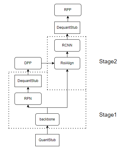
In some scenarios, users may need to deploy a model trained as a single unit in multiple segments. For example, in the two-stage detection model shown below, if DPP needs to run on the CPU and its output (roi) serves as input to RoiAlign, users must split the model into Stage1 and Stage2 according to the dashed-line boundaries for separate compilation and deployment. During hardware execution, the fixed-point data output by the backbone is directly used as input to RoiAlign.
Method
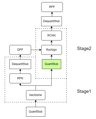
Model modification: As shown above, based on a normally quantization-trainable model, users need to insert a QuantStub after the segmentation boundary before
prepare_qat. Note that if usinghorizon_plugin_pytorch.quantization.QuantStub, the scale must be set toNone.QAT training: Train the modified model as a whole using standard quantization-aware training. The inserted QuantStub records the scale of Stage2 input data in its buffer.
Conversion to fixed-point: Use the
convertAPI to convert the trained QAT model to fixed-point, still treating it as a single unit.Splitting and compilation: Split the model according to the target hardware layout, then trace and compile each segment separately. Note that although Stage2 input is quantized during training, the example input used when tracing Stage2 must still be in floating-point format. The inserted QuantStub in Stage2 will assign the correct scale and perform quantization.
6.4.4.4. Operator Fusion
The training tool supports two main types of operator fusion: 1. BN absorption; 2. Fusion of Add and ReLU(6).
BN Absorption
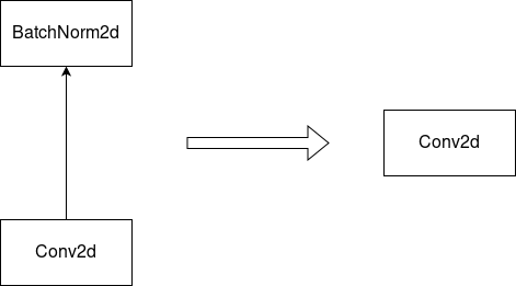
The purpose of absorbing BN is to reduce the model’s computational load. Since BN is a linear transformation, when BN appears together with Conv, the BN parameters can be absorbed into the Conv parameters, thereby eliminating the need to compute BN in the deployed model.
The absorption computation process is as follows:

By absorbing BN, Conv2d + BN2d can be simplified to Conv2d.
Fusion of Add and ReLU(6)
Unlike CUDA Kernel Fusion, which combines CUDA kernels to improve computation speed, the fusion supported by the training tool is more focused on the quantization level.
The BPU hardware is optimized for common model structures. When computing combinations such as Conv -> Add -> ReLU, it can maintain high precision during data transfer between operators, improving the overall numerical accuracy of the model. Therefore, during quantization, we can treat Conv -> Add -> ReLU as a single unit.
Since the training tool performs quantization modifications at the torch.nn.Module level, to treat Conv -> Add -> ReLU as a single unit during quantization, they must be merged into one Module.
In addition to preserving high precision in intermediate results, operator fusion also eliminates the need to convert intermediate results into low-precision representations, resulting in faster execution compared to non-fused versions.
(Since operator fusion improves both model accuracy and speed, all eligible parts should generally be fused.)
Implementation Principle
Thanks to FX’s ability to access the computation graph, the training tool can automatically analyze the model’s graph, match fusion patterns defined in advance, and perform fusion via submodule replacement. The example below illustrates this.
(BN absorption and Add/ReLU(6) fusion can be achieved using the same mechanism, so no distinction is needed during fusion.)
import torch
from torch import nn
from torch.quantization import DeQuantStub
from horizon_plugin_pytorch.quantization import QuantStub
from horizon_plugin_pytorch.quantization import fuse_fx


class ModelForFusion(torch.nn.Module):
    def __init__(
        self,
    ):
        super(ModelForFusion, self).__init__()
        self.quantx = QuantStub()
        self.quanty = QuantStub()
        self.conv = nn.Conv2d(3, 3, 3)
        self.bn = nn.BatchNorm2d(3)
        self.relu = nn.ReLU()
        self.dequant = DeQuantStub()

    def forward(self, x, y):
        x = self.quantx(x)
        y = self.quanty(y)
        x = self.conv(x)
        x = self.bn(x)
        x = x + y
        x = self.relu(x)
        x = self.dequant(x)

        return x


float_model = ModelForFusion()
fused_model = fuse_fx(float_model)

print(fused_model)
"""
ModelForFusion(
  (quantx): QuantStub()
  (quanty): QuantStub()
  (conv): Identity()
  (bn): Identity()
  (relu): Identity()
  (dequant): DeQuantStub()
  (_generated_add_0): ConvAddReLU2d(
    (conv): Conv2d(3, 3, kernel_size=(3, 3), stride=(1, 1))
    (relu): ReLU()
  )
)


def forward(self, x, y):
    quantx = self.quantx(x);  x = None
    quanty = self.quanty(y);  y = None
    _generated_add_0 = self._generated_add_0
    add_1 = self._generated_add_0(quantx, quanty);  quantx = quanty = None
    dequant = self.dequant(add_1);  add_1 = None
    return dequant
"""
As seen, after operator fusion, BN is absorbed into Conv, and Conv, Add, and ReLU are fused into a single module (_generated_add_0). The original submodules are replaced with Identity and are no longer invoked in the forward code.
(FX automatically replaces the x = x + y addition in the code with a Module named _generated_add_0 to support fusion and quantization operations.)
Supported Fusion Operators
Currently supported fusion operator combinations are defined in the following function:
import operator
import torch
from torch import nn
from horizon_plugin_pytorch import nn as horizon_nn


def register_fusion_patterns():
    convs = (
        nn.Conv2d,
        nn.ConvTranspose2d,
        nn.Conv3d,
        nn.Linear,
    )
    bns = (nn.BatchNorm1d, nn.BatchNorm2d, nn.BatchNorm3d, nn.SyncBatchNorm)
    adds = (
        nn.quantized.FloatFunctional.add,
        horizon_nn.quantized.FloatFunctional.add,
        torch.add,
        operator.add,  # i.e., the plus sign used in code
    )
    relus = (nn.ReLU, nn.ReLU6, nn.functional.relu, nn.functional.relu6)

    for conv in convs:
        for bn in bns:
            for add in adds:
                for relu in relus:
                    # conv bn
                    register_fusion_pattern((bn, conv))(ConvBNAddReLUFusion)

                    # conv relu
                    register_fusion_pattern((relu, conv))(ConvBNAddReLUFusion)

                    # conv add
                    register_fusion_pattern((add, conv, MatchAllNode))(
                        ConvBNAddReLUFusion
                    )  # conv output as first input to add
                    register_fusion_pattern((add, MatchAllNode, conv))(
                        ConvBNAddedReLUFusion
                    )  # conv output as second input to add

                    # conv bn relu
                    register_fusion_pattern((relu, (bn, conv)))(
                        ConvBNAddReLUFusion
                    )

                    # conv bn add
                    register_fusion_pattern((add, (bn, conv), MatchAllNode))(
                        ConvBNAddReLUFusion
                    )
                    register_fusion_pattern((add, MatchAllNode, (bn, conv)))(
                        ConvBNAddedReLUFusion
                    )

                    # conv add relu
                    register_fusion_pattern((relu, (add, conv, MatchAllNode)))(
                        ConvBNAddReLUFusion
                    )
                    register_fusion_pattern((relu, (add, MatchAllNode, conv)))(
                        ConvBNAddedReLUFusion
                    )

                    # conv bn add relu
                    register_fusion_pattern(
                        (relu, (add, (bn, conv), MatchAllNode))
                    )(ConvBNAddReLUFusion)
                    register_fusion_pattern(
                        (relu, (add, MatchAllNode, (bn, conv)))
                    )(ConvBNAddedReLUFusion)
6.4.4.5. Adaround (Experimental Feature)
Adaround is a state-of-the-art post-training quantization (PTQ) method that improves quantization accuracy over traditional rounding-to-nearest strategies by learning layer-wise whether to round weights up or down. In our experiments, Adaround effectively enhances calibration accuracy with minimal performance overhead across various tasks (e.g., classification, segmentation, BEV), serving as a valuable complement to existing calibration workflows.
Basic Principle
Adaround aims to reduce quantization error by learning a better rounding scheme, and thus targets operators with weights. Currently, only Conv and Linear layers are supported. Adaround optimizes Conv/Linear layers sequentially in topological order, learning an up/down rounding mask by minimizing per-operator quantization error, and finally modifies the weights in-place to complete the optimization.
Interface Definition
def weight_reconstruction(
    calib_model: torch.nn.Module,
    batches: Union[list, tuple, DataLoader],
    batch_process_func: Callable = None,
    custom_config_dict: dict = None,
):
    pass
Here, custom_config_dict contains configuration parameters related to Adaround:
    custom_config_dict = {
        "num_batches": 10,
        "num_steps": 100,
        "exclude_prefix": [],
        "warm_up": 0.2,
        "weight": 0.01,
        "b_range": [20, 2],
    }
num_batches: Only effective when the input data is a DataLoader. It specifies the number of batches from the DataLoader used for Adaround optimization. If the input is a list/tuple, this parameter is ignored, and all batches in the list will be used. The default value of 10 is generally sufficient.
num_steps: Number of optimization steps per Conv/Linear layer. Larger values generally yield better theoretical results. This is the primary hyperparameter you should focus on when tuning Adaround.
exclude_prefix: If certain modules should not be optimized by Adaround, add their prefixes here. All modules with names starting with the specified prefix will be excluded. In most of our experiments, this parameter is unnecessary, as Adaround consistently improves calibration accuracy. However, in rare cases (e.g., certain detection models), optimizing the detection head may degrade accuracy. In such cases, use this parameter to filter out specific layers.
warm_up: A value between [0, 1], indicating the warm-up ratio. During the first warm_up * num_steps steps, no regularization is applied to the rounding process, allowing optimization to focus purely on accuracy. This has minor impact on performance; the default value of 0.2 is typically sufficient.
weight: Regularization coefficient for the round loss. A larger value strengthens the dominance of round loss in the total loss. This is a secondary tuning parameter, with a default value of 0.01. It can be adjusted around this value (e.g., 0.1, 0.001) based on relative loss magnitudes.
b_range: b controls the smoothness of the round loss, and b_range defines its range. Usually, no adjustment is needed; the default [20, 2] is recommended. This means b starts at 20 and linearly decays to 2 over the optimization steps.
The product batch_size * num_steps represents the effective number of samples processed per operator during optimization (with possible duplicates due to random sampling). A recommended range is 10,000–20,000.
1. `num_steps` **is the main parameter affecting Adaround accuracy. When tuning hyperparameters, you generally only need to focus on this parameter.**

2. In our experiments, Adaround consistently improves calibration accuracy across most tasks by simply adjusting `num_steps`. However, in detection tasks, it may be necessary to carefully set `exclude_prefix` to exclude certain layers in the detection head to achieve accuracy gains. If Adaround degrades calibration accuracy in your detection task, we recommend switching to Quantization-Aware Training (QAT) for better quantization performance.
For additional parameter details, please refer to the interface’s docstring.
Usage
We support two data input methods.
list/tuple (Recommended)
Since this interface frequently accesses data, we recommend packaging your data into a list or tuple. In this case, all data will be moved to GPU/CPU memory (depending on the model’s device), reducing memory access bottlenecks caused by repeated data loading. Compared to using a DataLoader, this method offers significant performance advantages.
# First perform normal calibration
calib_model = horizon.quantization.prepare_qat_fx(float_model)
calib_model.eval()
horizon.quantization.set_fake_quantize(
    calib_model, horizon.quantization.FakeQuantState.CALIBRATION
)
for image, label in dataloader:
    calib_model(image)

# Prepare data for Adaround
batches = []
n = 0
for image, label in dataloader:
    if n >= 10:
        break
    batches.append(image)
    n += 1

# Custom Adaround configuration: exclude the "head" module
custom_config_dict = {"num_steps": 100, "exclude_prefix": ["head",]}

horizon.quantization.weight_reconstruction(
    calib_model,
    batches,
    None, # batch_process_func; keep default since batches already meet requirements
    custom_config_dict,
)

# Evaluation
calib_model.eval()
horizon.quantization.set_fake_quantize(
    calib_model, horizon.quantization.FakeQuantState.VALIDATION
)
for image, label in eval_dataloader:
    pred = calib_model(image)
    pass
torch.utils.data.DataLoader
Although the list/tuple approach offers better performance, it requires loading all calibration data into memory, which may be demanding for some hardware. Therefore, we also support directly passing a torch DataLoader for easier use in certain scenarios. Since DataLoader loads data only when needed, it uses less memory but incurs higher memory access overhead. In our experiments, the performance of the DataLoader approach lags significantly behind the list/tuple method; please use it judiciously.
# First perform normal calibration
calib_model = horizon.quantization.prepare_qat_fx(float_model)
calib_model.eval()
horizon.quantization.set_fake_quantize(
    calib_model, horizon.quantization.FakeQuantState.CALIBRATION
)
for image, label in dataloader:
    calib_model(image)

# Custom Adaround configuration: set num_batches to 16, meaning only 16 batches from the dataloader will be used
custom_config_dict = {"num_batches": 16, "num_steps": 100, "exclude_prefix": ["head",]}

horizon.quantization.mix_calibration(
    calib_model,
    dataloader, # pass dataloader directly
    lambda x: x[0], # batch_process_func; index to extract image since batch is Tuple[image, label]
    custom_config_dict,
)

# Evaluation
calib_model.eval()
horizon.quantization.set_fake_quantize(
    calib_model, horizon.quantization.FakeQuantState.VALIDATION
)
for image, label in eval_dataloader:
    pred = calib_model(image)
    pass
6.4.4.6. Automatic Calibration (Experimental Feature)
The quantization-aware training toolkit has integrated various calibration strategies such as MSE, KL, percentile, min-max, etc. For most models, MSE achieves satisfactory calibration accuracy. However, if you have expertise and wish to explore higher-accuracy calibration pipelines, the current calibration interface may not suffice. To address this, we have developed an automatic calibration interface that allows you to define searchable calibration strategies and hyperparameters, enabling layer-by-layer search for optimal quantization parameters based on model output similarity.
This interface differs from the Mix Observer in our Calibration pipeline in the following ways:
When searching for quantization parameters of an operator, Mix Observer uses only the output similarity of that single operator as the evaluation metric. In contrast, this interface uses the final model output similarity as the metric.
When optimizing a specific operator, Mix Observer keeps preceding operators in floating-point mode, ignoring accumulated quantization error. This interface, however, keeps all preceding activations and weights quantized during the search.
Our ablation studies show that both aspects contribute positively to calibration accuracy.
Note that due to its layer-by-layer search strategy and reliance on final model output similarity, this method is computationally expensive and time-consuming.
Basic Principle
Record the outputs of all DeQuantize operators in the floating-point model.
Traverse each quantizable operator in topological order:
When calibrating an operator, quantize its weight (if any) and activation, iterate over user-specified calibration strategies, and record the corresponding DeQuantize outputs.
Compute the L2 distance between quantized and floating-point outputs, and update the optimal quantization parameters.
After evaluating all calibration strategies, apply the best parameters to the current operator and proceed to the next.
Interface Definition
def auto_calibrate(
    calib_model: torch.nn.Module,
    batches: Union[list, tuple, DataLoader],
    num_batches: int = 10,
    batch_process_func: Callable = None,
    observer_list: list = ("percentile", "mse", "kl", "min_max"),
    percentile_list: list = None,
):
    pass
For further interface details, please refer to the docstring.
Usage
We support two data input methods.
list/tuple (Recommended)
Due to frequent data access, we recommend packaging data into a list or tuple. This reduces memory access bottlenecks by pre-loading all data into GPU/CPU memory. Compared to DataLoader, this method offers significant performance benefits.
calib_model = horizon.quantization.prepare_qat_fx(float_model)
batches = []
n = 0
for image, label in dataloader:
    if n >= 10:
        break
    batches.append(image)
    n += 1

horizon.quantization.auto_calibration(
    calib_model,
    batches,
    10, # num_batches; ignored in this mode, default is fine. All batches in list are used.
    None, # batch_process_func; default is sufficient as data is already in correct format
    ["percentile", "min_max"], # custom list of calibration strategies to search
    [99.99, 99.999, 99.9995, 99.9999], # custom percentile values
)

# Evaluation
calib_model.eval()
horizon.quantization.set_fake_quantize(
    calib_model, horizon.quantization.FakeQuantState.VALIDATION
)
for image, label in eval_dataloader:
    pred = calib_model(image)
    pass
torch.utils.data.DataLoader
While the list/tuple method offers better performance, it requires loading all calibration data into memory, which may not be feasible on all devices. Hence, we also support directly passing a torch DataLoader for convenience in certain use cases. DataLoader loads data on-demand, reducing memory footprint but increasing memory access overhead. In our experiments, the DataLoader approach performs significantly worse than the list/tuple method; please use it cautiously.
calib_model = horizon.quantization.prepare_qat_fx(float_model)

horizon.quantization.auto_calibration(
    calib_model,
    dataloader, # pass dataloader directly
    10, # num_batches; only use 10 batches from dataloader for calibration
    lambda x: x[0], # batch_process_func; extract image from Tuple[image, label]
    ["percentile", "min_max"], # custom list of calibration strategies
    [99.99, 99.999, 99.9995, 99.9999], # custom percentile values
)

# Evaluation
calib_model.eval()
horizon.quantization.set_fake_quantize(
    calib_model, horizon.quantization.FakeQuantState.VALIDATION
)
for image, label in eval_dataloader:
    pred = calib_model(image)
    pass